
The Map: The Whole of PyTorch on One Page


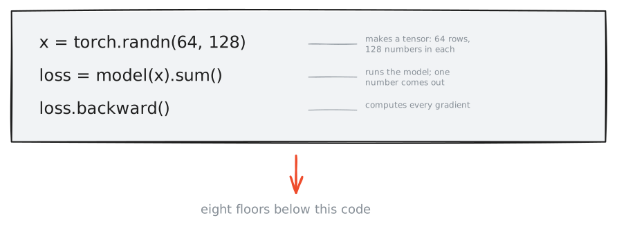
Figure 1. the program this whole series is about.
You have typed something like this a thousand times. This series exists so that, by its end, you know everything these lines do. All of it: the Python they touch, the C++ they land in, the graph they record, the kernels they choose, the memory they use, and the two clocks they run on. Each of those words gets a plain meaning on its floor below.
This is Part 0, the map. First we go down through all the layers once, fast. Then we draw the territory. Then twelve ideas that make the rest of the codebase predictable. Then how this series works, and how to read it. Nothing here gets its full story. Everything here gets a place, and every full story has a numbered part waiting for it.
One promise before we start. Every measured number in this series comes from a small script you can run yourself, linked right where the number appears. I measured these on an Apple M3 Max laptop with torch 2.11.0 [1]. Your numbers will differ. The pattern they make will not.
The fall
PyTorch is deep. Between your keyboard and the chip there are eight levels. I will call them floors, and this meter shows all of them. It returns through the whole series, so you always know how deep you are.
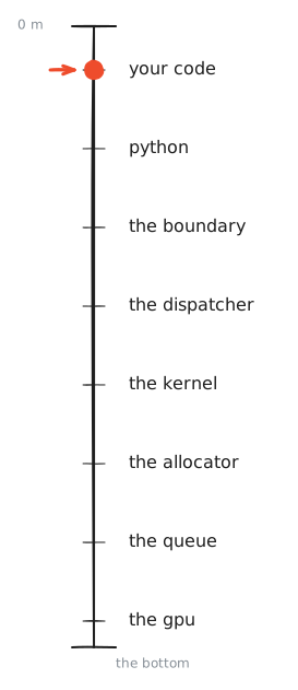
Figure 2. the depth meter. the orange dot marks where you are.
The fastest way to learn a building is to go down through it once without stopping. That is this section.
Floor one: python
floor 2 of 8: python · full story: Part 5, The Machinery
torch.randn looks like a Python function. Ask Python what it
actually is:
>>> type(torch.randn)
<class 'builtin_function_or_method'>
Python gives that type only to functions written in compiled code. Compiled code means: code that was translated to machine instructions before you ever installed it, so there is no Python body inside it to read, and no line for your debugger to stop on.
So where do those machine instructions live? In shared libraries. A shared library is a file of compiled code that a program loads while it runs. They sit inside the torch package on your disk, and you can look at them (proof):
torch._C -> _C.cpython-312-darwin.so  (49 KB, the loader)
libtorch_cpu.dylib        206.5 MB   (tensors and kernels)
libtorch_python.dylib      28.5 MB   (the python side of the border)
p0_the_library.py · the proof, ready to read or run
"""Proof: where the compiled part of pytorch actually lives.

torch._C is a thin compiled stub; the weight of the framework is in
the shared libraries next to it. Prints the files and their sizes.
"""
import glob
import os
import torch

stub = torch._C.__file__
print(f"torch {torch.__version__}")
print(f"torch._C -> {os.path.basename(stub)}  "
      f"({os.path.getsize(stub)/1024:.0f} KB stub)")
libdir = os.path.join(os.path.dirname(stub), "lib")
for lib in ["libtorch_cpu.dylib", "libtorch_python.dylib"]:
    p = os.path.join(libdir, lib)
    if os.path.exists(p):
        print(f"{lib:24s} {os.path.getsize(p)/1024/1024:6.1f} MB")
Read the sizes, and then look at them:
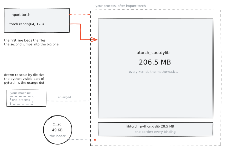
Figure 3. drawn to scale by file size. the part of pytorch that python can see is the orange dot.
The part of PyTorch you can see from Python is a 49 KB file whose
only job is to load the other two. The real body is 235 MB of
compiled code. import torch brings it into your process, and
after that, calling torch.randn means jumping into that body.
Today we only need to know these files exist.
This is the first honest surprise of the codebase: the Python you write all day is the smallest layer of it.
The boundary
floor 3 of 8: the boundary · full story: Part 5, The Machinery
The call leaves Python at once. Where does it land?
In a C++ function named THPVariable_randn, inside that 28.5 MB
library from the last floor. And here is a strange fact you can
keep: this function does not exist in the PyTorch repository. Clone
the repo, search for the name, and you find nothing. A program
writes this function during the build, together with thousands of
its siblings. Idea 4 below explains why, and Part 5 shows the
program that does the writing.
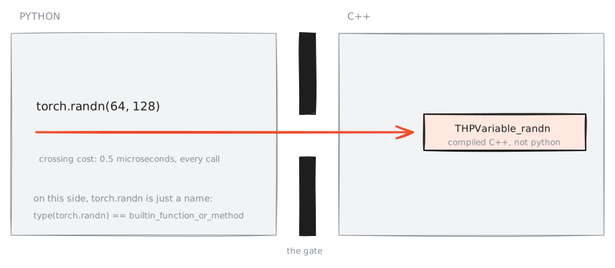
Figure 4. the border between the two languages. every tensor operation crosses it.
Crossing this border costs time. To see the cost alone, time the smallest possible operation, where almost no arithmetic hides it (proof):
add, 1 element   :    0.538 microseconds per call
add, 4M elements :  337.264 microseconds per call
p2_dispatch_cost.py · the proof, ready to read or run
"""Proof: the fixed cost of one eager op, and why size hides it.

Times the same `a + b` at two sizes. The one-element add is nearly
pure machinery (dispatch, wrapping, allocation); the 4M-element add is
nearly pure arithmetic. CPU, single process.
"""
import time
import torch

def per_op_us(a, b, iters):
    # warmup
    for _ in range(2000):
        a + b
    t0 = time.perf_counter()
    for _ in range(iters):
        a + b
    return (time.perf_counter() - t0) / iters * 1e6

tiny = per_op_us(torch.ones(1), torch.ones(1), 200_000)
big_n = 4_000_000
big = per_op_us(torch.ones(big_n), torch.ones(big_n), 2_000)

print(f"torch {torch.__version__}, cpu")
print(f"add, 1 element   : {tiny:8.3f} us/op")
print(f"add, 4M elements : {big:8.3f} us/op")
print(f"machinery share of the tiny op: ~all of it")
print(f"ops/sec you can issue from python: {1e6/tiny:,.0f}")

# The sweep behind the toll meter: the same add at twelve sizes,
# 1 to 4M elements in powers of four. Every dot on the widget's
# axis is one line of this output.
import json
sweep = []
for k in range(12):
    n = 4 ** k
    iters = max(1_000, min(200_000, 40_000_000 // max(n, 1)))
    us = per_op_us(torch.ones(n), torch.ones(n), iters)
    sweep.append({"n": n, "us": round(us, 3)})
    print(f"add, {n:>9,} elements : {us:9.3f} us/op")
print("JSON_SWEEP=" + json.dumps(sweep))
The one-element add does almost no math. So its 0.54 microseconds is almost pure crossing cost: leave Python, check the arguments, build the result object, return. Half a microsecond sounds like nothing. It means Python can issue at most about 1.9 million operations per second, and a single training step contains thousands of operations. Keep this number. It returns in Idea 6.
The dispatcher
floor 4 of 8: the dispatcher · full story: Part 5, The Machinery
Under the border, the call reaches the strangest machine in PyTorch: the dispatcher. The dispatcher is the router that decides, for every operation, which pieces of code run and in what order.
Look at what it must decide. Your three lines never said "record
gradients". No if statement in your code turns that on. Yet
somewhere, something decided that this matrix multiplication should
be remembered for backward(). That something is the dispatcher.
Every operation passes down through a fixed stack of layers. Each
layer can act on the call, change it, or let it pass unchanged.
Autograd, the part of PyTorch that computes gradients, is one such
layer. Mixed precision is another. On this run, only autograd is
awake.
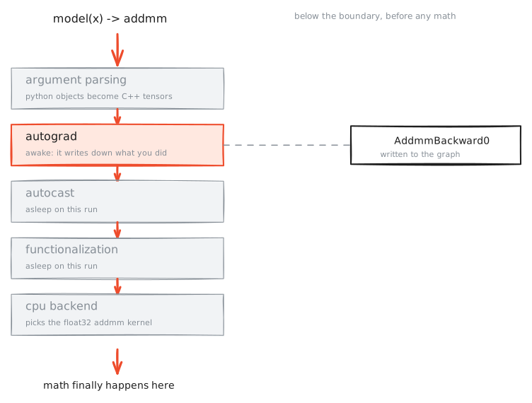
Figure 5. four layers touch your call before any arithmetic starts. only the highlighted one is awake today.
The kernel
floor 5 of 8: the kernel · full story: Part 8, Kernels & Hardware
At the bottom of the stack, one concrete function is chosen. Chosen
is the right word. This torch build has 3,677 registered operation
names (proof prints
the count), and a name is not a function body. The operation addmm,
the matrix multiplication behind model(x), has separate bodies
for CPU and for each kind of GPU, for each data type, for dense and
for sparse tensors. A body like this, written for one device and
one data type, is called a kernel. The dispatcher's last job is to
pick one:
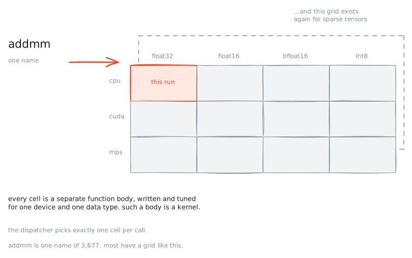
Figure 6. one name, a grid of bodies. the dispatcher picks exactly one cell per call.
p4_micro_proofs.py · the proof, ready to read or run
"""Micro-proofs quoted in Part 0: storage sharing, view errors,
mutation rewriting history, the no_grad layer, float32 absorption."""
import torch

print(f"torch {torch.__version__}\n")

# 1. a tensor is a window over storage
x = torch.arange(6, dtype=torch.float32)
v = x.view(2, 3)
print("same bytes under both:", x.data_ptr() == v.data_ptr())
print("v.stride():", v.stride(), " v.t().stride():", v.t().stride())
try:
    v.t().view(-1)
except RuntimeError as e:
    print("v.t().view(-1) ->", str(e).split(".")[0])

# 2. mutation rewrites the recorded program
a = torch.ones(3, requires_grad=True)
y = a * 2
print("\nbefore add_:", type(y.grad_fn).__name__)
y.add_(1)
print("after  add_:", type(y.grad_fn).__name__)

# 3. no_grad removes one dispatcher layer
with torch.no_grad():
    z = a * 2
print("\ninside no_grad, grad_fn:", z.grad_fn)

# 4. float32 absorbs small numbers
t = torch.tensor(1e8)
print("\n(1e8 + 1) - 1e8 in float32 =", ((t + 1) - t).item())

# 5. the size of the operation list (idea 3)
print("\nregistered operation names:",
      len(torch._C._dispatch_get_all_op_names()))
The full list of operations lives in one file in the repository:
native_functions.yaml [2].
Its sibling
derivatives.yaml [3]
lists the derivative of each operation. Everything else grows from
these two files. No other file in the repository tells you as much
per line.
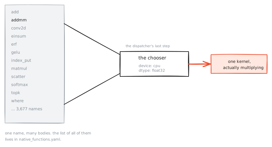
Figure 7. 3,677 names on the left. one function body on the right. the funnel is the dispatcher's last job.
One floor down sits memory. torch.randn(64, 128) needs 32,768
bytes: 64 rows times 128 numbers times 4 bytes per number. On the
CPU this is an ordinary allocation. On a GPU it is not. There,
PyTorch runs its own allocator, a keeper of memory that asks the
GPU driver for large blocks once and then reuses them, because
asking the driver every time is slow. This allocator decides when
you run out of memory and what the error means. Part 4 examines it.
The two clocks
floor 7 of 8: the queue · full story: Part 4, Seeing PyTorch
Here the story splits in two. What follows is the single most useful performance fact in PyTorch.
On a GPU, your Python line does not do the work. It requests the work, and the request returns at once. The GPU does the work on its own clock, while Python continues. I measured it on this machine's GPU (proof):
time to request 50 matrix multiplications :   1.58 ms
time until the work was actually done     :  73.83 ms
python was free during                    :  72.25 ms  (98%)
p3_two_timelines.py · the proof, ready to read or run
"""Proof: the CPU runs ahead of the GPU.

Queues 50 large matmuls on the MPS device and measures two times:
how long Python took to *ask* for the work, and how long the work
actually took. The difference is the gap the chapter draws.
"""
import time
import torch

assert torch.backends.mps.is_available(), "needs an Apple-silicon GPU"
dev = torch.device("mps")

a = torch.randn(2048, 2048, device=dev)
b = torch.randn(2048, 2048, device=dev)
for _ in range(5):          # warmup
    (a @ b)
torch.mps.synchronize()

t0 = time.perf_counter()
for _ in range(50):
    c = a @ b
t_queue = time.perf_counter() - t0
torch.mps.synchronize()
t_done = time.perf_counter() - t0

print(f"torch {torch.__version__}, mps")
print(f"time to queue 50 matmuls : {t_queue*1e3:8.2f} ms")
print(f"time until work finished : {t_done*1e3:8.2f} ms")
print(f"python was free for      : {(t_done-t_queue)*1e3:8.2f} ms ({(t_done-t_queue)/t_done:.0%} of the wall time)")

# The three ways to read the loss, measured, for the two-clocks
# widget: never, once at the end, after every step.
import json
def run_mode(mode, iters=50):
    for _ in range(5):
        (a @ b)
    torch.mps.synchronize()
    t0 = time.perf_counter()
    t_free = 0.0
    for i in range(iters):
        c = a @ b
        if mode == "every":
            c[0, 0].item()
    t_q = time.perf_counter() - t0
    if mode == "once":
        c[0, 0].item()
    torch.mps.synchronize()
    total = time.perf_counter() - t0
    return {"mode": mode, "queue_ms": round(t_q * 1e3, 2),
            "total_ms": round(total * 1e3, 2),
            "free_ms": round((total - t_q) * 1e3, 2)}

modes = [run_mode(m) for m in ("never", "once", "every")]
for m in modes:
    print(f"read {m['mode']:>5}: total {m['total_ms']:8.2f} ms, "
          f"python busy {m['queue_ms']:8.2f} ms")
print("JSON_MODES=" + json.dumps(modes))
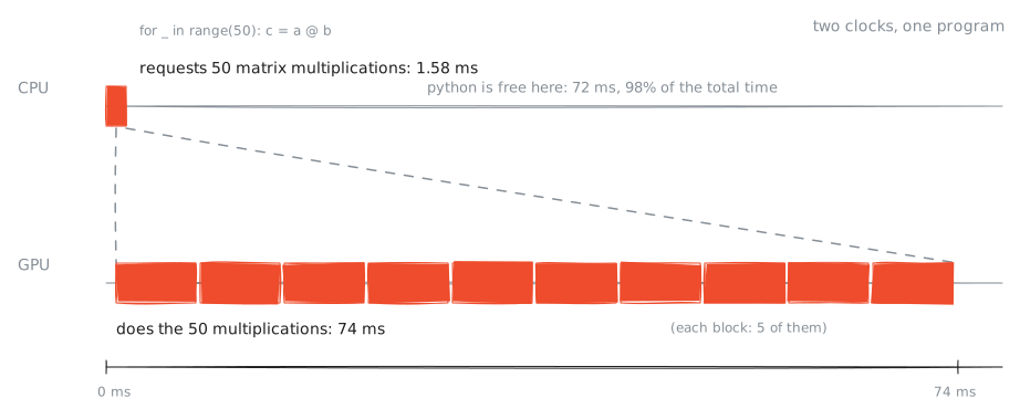
Figure 8. two clocks, one program. the cpu requested everything in the first two milliseconds; the gpu needed seventy-two more to finish.
Python asked for all fifty multiplications in under two milliseconds, then waited, free, while the GPU computed for another seventy-two. On the CPU there is no such split; the math happens before your line returns. On any accelerator, the split is the normal state of the program.
This is why eager PyTorch is fast enough to use: Python runs ahead
and the GPU never waits for it. It is also why simple timing code
gives wrong answers, and why one loss.item() inside a training
loop can slow the whole step. .item() needs the actual number. The
number sits at the end of a queue of work the GPU has not finished
yet, so Python must stop and wait for the whole queue:
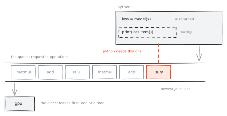
Figure 9. the queue between the two clocks. the number python asked for is the last ticket, so every ticket ahead of it must finish first.
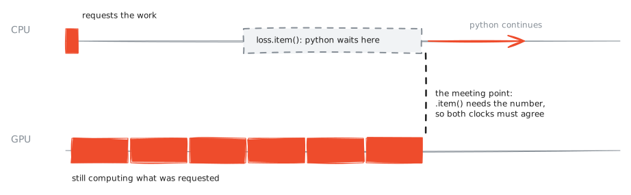
Interactive 1. the two clocks, measured. choose how often the loop reads the loss; the lanes show who waits, and for how long. This is a live instrument in the original post; the still drawing stands in here.
Part 4 teaches honest measurement on top of exactly this picture.
The turn
floor 4 of 8: the autograd layer · full story: Part 2, Autograd
Line three: loss.backward(). Nothing so far explains how this
line can work. The forward computation is over. How does PyTorch
know what to differentiate?
It knows because the forward pass had a second job. Every time an
operation passed the autograd layer of the dispatcher, a small
record was written: which operation ran, and which recorded steps
produced its inputs. Records that point at
records form a graph, and that word here always means exactly this
recorded structure. By the time loss exists, its graph exists
too (proof):
loss.grad_fn     = SumBackward0
SumBackward0
  AddmmBackward0
    AccumulateGrad
p1_graph_chain.py · the proof, ready to read or run
"""Proof: loss.backward() walks a graph that forward quietly recorded.

Builds the chapter's three-line program and prints the autograd graph
that exists before backward is ever called.
"""
import torch
import torch.nn as nn

torch.manual_seed(0)
model = nn.Sequential(nn.Linear(128, 256), nn.ReLU(), nn.Linear(256, 10))

x = torch.randn(64, 128)
loss = model(x).sum()

print(f"torch {torch.__version__}")
print(f"x.grad_fn        = {x.grad_fn}")
print(f"loss.grad_fn     = {type(loss.grad_fn).__name__}")

node, depth = loss.grad_fn, 0
while node is not None and depth < 10:
    print("  " * depth + type(node).__name__)
    nexts = [n for n, _ in node.next_functions if n is not None]
    node = nexts[0] if nexts else None
    depth += 1
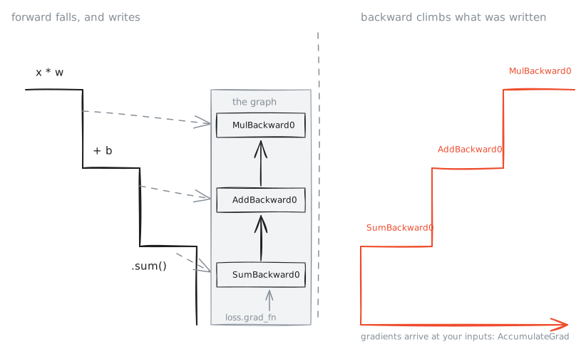
Figure 10. the forward pass goes down and writes the graph. backward climbs exactly what was written, and nothing else.
backward() invents nothing. It walks the graph from the loss back
to your inputs, runs each recorded derivative, and stores the
results in .grad. The walk ends at AccumulateGrad, the record
that does the storing. And it starts nowhere else: x.grad_fn is
None, because x was created directly, not computed.
One question should bother you here. A derivative needs values. The derivative of a matrix multiplication needs the matrices that were multiplied, and the forward pass is long over. Write the derivative out and the need is visible:
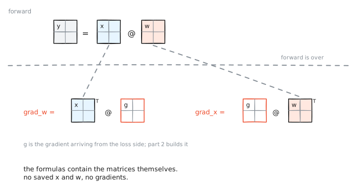
Figure 11. the derivative of x @ w, written out. the formulas contain x and w themselves; whatever forward used, backward needs again.
So where are they? They were saved, next to the records, during the forward pass:
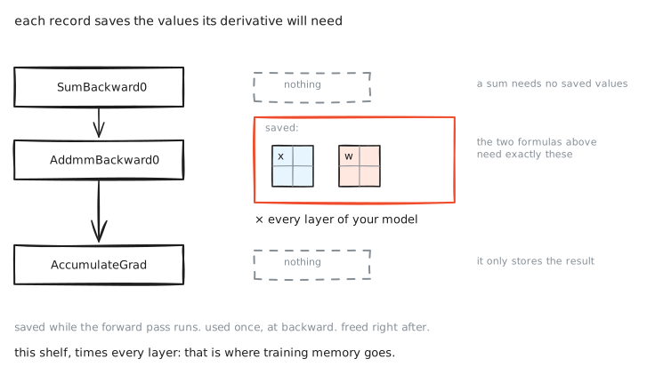
Figure 12. what each record kept. this is where the memory of a training run actually goes.
So the forward pass silently decides how much memory training costs. Part 2 shows the exact saving rules. Part 4 shows how to watch it happen. And a method called activation checkpointing trades that memory for extra compute; it has its own chapter in Part 2.
Carry one sentence out of this section: backward can only walk what forward wrote. It sounds small. In Part 9 it becomes the rule that decides which GPUs in a cluster must talk to each other.
That was the whole fall: a name, a border, a stack of layers, a chosen kernel, a keeper of memory, two clocks, and a graph that is walked backward. Now the territory, properly.
The territory
PyTorch is built in layers, and each layer speaks only to its neighbors. Every box below is at least one part of this series.
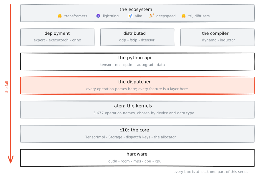
Figure 13. the whole system on one sheet. the orange line on the left is the path we just took.
The same territory, seen as folders in the repository. If you ever open the codebase, this is the map that stops you from being lost:
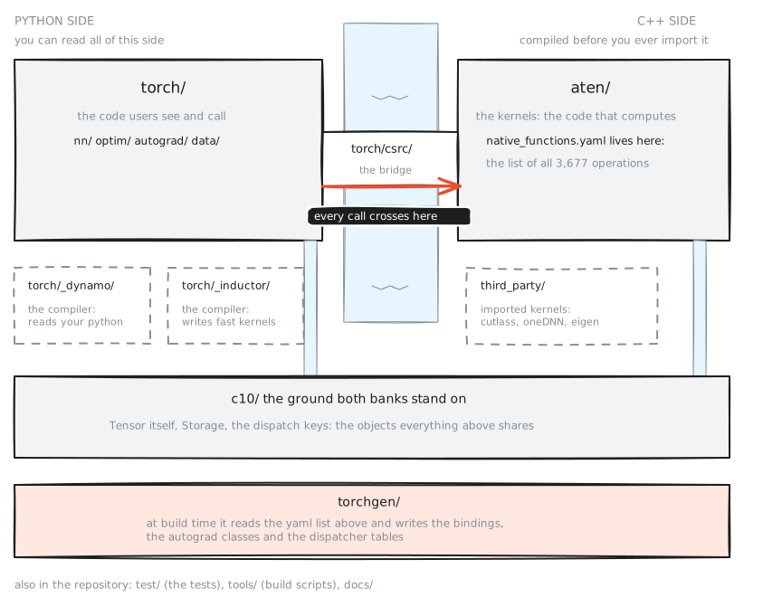
Figure 14. the repository as two river banks. the river is the boundary from figure 4; torch/csrc/ is its one bridge; and both banks stand on the same ground, c10/, where Tensor and Storage themselves live.
Three facts about this map save you weeks. First: torch/ is
plain Python, and you can read every file in it today. Second:
aten/ and c10/ are C++; the tensors, the kernels and the
dispatcher live there, and torch/csrc/ is the single bridge that
connects the two languages. Third: torchgen/ is the program from
the boundary floor, the one that writes code during the build. The
repository you read is the input. The library you run is the
output. That is why searching the repository for
THPVariable_randn finds nothing:
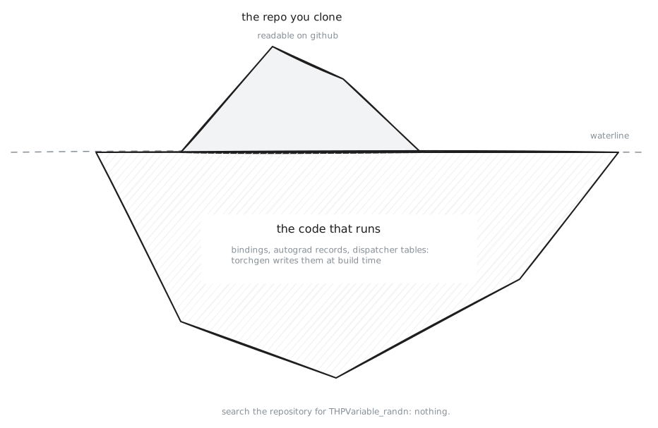
Figure 15. the repository is the part above the waterline. the code your process runs is the larger part below it.
Above the core sits the ecosystem. It looks endless, but it has a simple shape: every library attaches to PyTorch at a specific, nameable place. Know the attachment places and you know the ecosystem.
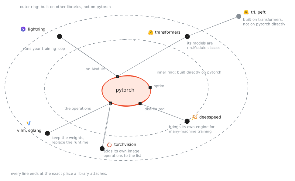
Figure 16. every line points at the exact place a library attaches. trl and peft sit on the outer ring: they build on transformers, not on pytorch.
Read the picture from the center out. transformers builds its
models as nn.Module classes, so if you understand Part 3, you can
read its source. deepspeed replaces the distributed engine, so
its home is Part 9. vllm and sglang keep the model weights and
replace the runtime around them. And trl and peft do not touch
PyTorch directly at all; they build on transformers.
The whole ecosystem fits in one table. The second column names the place in the PyTorch repository where each family attaches:
| attaches at | the pytorch side | who | what they keep, what they bring |
|---|---|---|---|
| nn.Module | torch/nn/ |
transformers, diffusers, timm | models are Modules; torch runs them |
| the training loop | torch/autograd/ torch/optim/ |
lightning, accelerate | torch stays the engine; they drive it |
| the distributed engine | torch/distributed/ |
deepspeed | swaps the engine, brings ZeRO |
| the eager runtime | torch/nn/ torch/library.py |
vllm, sglang, TensorRT-LLM | keep the weights, replace the runtime, each with a csrc/ of its own kernels |
| the operation list | aten/ torch/library.py |
flash-attention, torchvision ops | new names on the list |
| two floors at once | torch/autograd/ + transformers |
unsloth | trains through transformers, brings its own Triton kernels |
| only the weights | none; the weights file | TEI, llama.cpp, MLX | left pytorch, kept the weights; llama.cpp re-encodes them to GGUF |
Two rows of the table deserve pictures. The first is the eager runtime, the thing the serving engines replace:
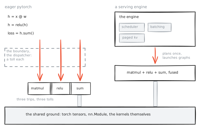
Figure 17. two ways to run one model. the engines replace the loop in the middle; the ground is shared.
The second is Triton, the kernel language that appears through the whole table: PyTorch's compiler writes it, and libraries bring their own:
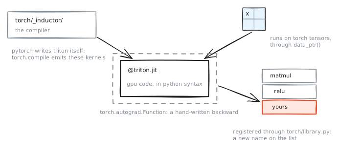
Figure 18. triton and pytorch. the compiler writes triton itself; hand-written kernels run on torch tensors and join the list.
Read the table downward and less of PyTorch survives each row. The last row keeps nothing but the weights file. That is the quiet law of the ecosystem: the weights outlive the runtime. Part 10 walks these attachment points one by one.
The twelve ideas
Most of PyTorch is not thousands of separate decisions. It is a small set of ideas, applied everywhere. These twelve make the rest of the codebase predictable before you read it. Each one returns later as a full chapter or part. Each one comes with runnable evidence now; the small proofs share one script (proof).
1. A tensor is a window over storage
full story: Part 1, Tensor
A tensor does not hold numbers. It holds a description of where to look: a pointer into one flat block of memory, the sizes of each dimension, and the strides. A stride is the number of steps to move in that flat block to reach the next element of a dimension. Two tensors can look completely different and read the same bytes:
>>> x = torch.arange(6.); v = x.view(2, 3)
>>> x.data_ptr() == v.data_ptr()   # same address in memory
True
>>> v.stride(), v.t().stride()     # transpose swapped the strides
((3, 1), (1, 3))
The transpose moved no data. It swapped two numbers in the
description. Some descriptions are impossible to write down, and
that is exactly why v.t().view(-1) raises an error while
reshape silently copies the data instead. Part 1 opens with this
puzzle and solves it completely.
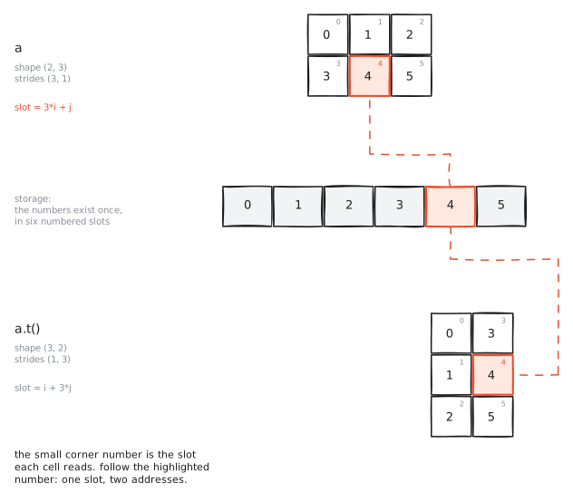
Interactive 2. six numbers, one storage. shape and strides decide which slot every cell reads; view(-1) exists only when the walk matches storage order. This is a live instrument in the original post; the still drawing stands in here.
2. Autograd records a program you never wrote
full story: Part 2, Autograd
In your code, y is one name, and you overwrite it freely. Line
two destroys the value line one made. The graph cannot afford
that: backward will need every step. So autograd writes one record
per change, and no record is ever overwritten. Watch the record
change as y does:
>>> a = torch.ones(3, requires_grad=True)
>>> y = a * 2
>>> type(y.grad_fn).__name__
'MulBackward0'
>>> y.add_(1)                      # change y in place
>>> type(y.grad_fn).__name__
'AddBackward0'
>>> y[0] = 9                       # overwrite one slot
>>> type(y.grad_fn).__name__
'CopySlices'
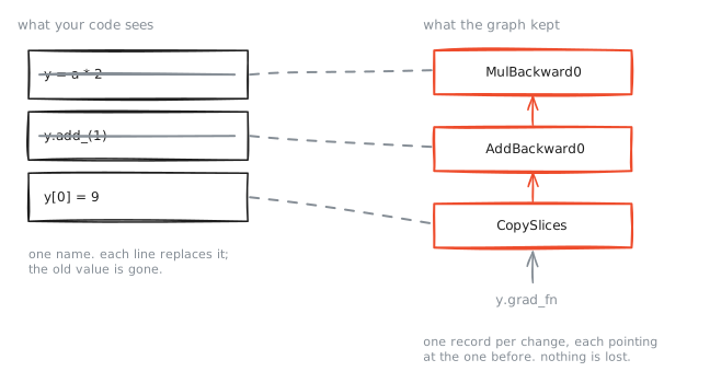
Figure 19. your code keeps one value and destroys the past. the graph keeps every step: one record per change, nothing overwritten.
Three statements, three records, one chain. y.grad_fn always
holds the newest record, and each record points at the one before
it, so the whole history stays reachable. That history is the
program you never wrote. The machinery that keeps it correct under
every kind of in-place change has real depth, and it is one of the
best chapters of Part 2.
3. One list of operations is the whole interface
full story: Part 5, The Machinery
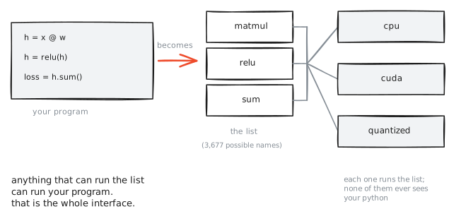
Figure 20. the code on the left never reaches a device. only the list does.
The 3,677 registered names are PyTorch's real interface. Each
backend implements its share of them. The compiler rewrites
programs made of them: torch.compile reads the list your program
became and returns a shorter one, where a matrix multiplication
and the add after it can fuse into one addmm, and a chain of
small elementwise operations becomes one generated kernel. Export
formats store them: torch.export writes the list to disk as a
graph of exactly these names, and an ONNX file is the same idea
with each name translated into ONNX's vocabulary. Quantization
replaces them: the float32 matmul is swapped for an int8 body, the
same place on the list, different arithmetic. When you meet a new
PyTorch technology, ask one question first: what does it do to the
operations? The answer usually explains the whole design.
4. PyTorch writes most of its own code
full story: Part 5, The Machinery
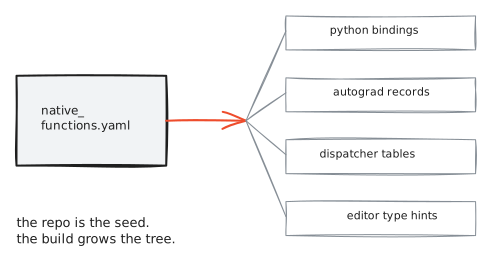
Figure 21. one yaml file in, thousands of functions out, at every build.
native_functions.yaml declares every operation.
derivatives.yaml declares every derivative. At build time,
torchgen/ reads both and writes the Python bindings, the autograd
record classes and the dispatcher tables. This is why searching the
repository for a function you just called can find nothing: you
searched the input of the build, and the function is in the output.
People who work on PyTorch read the yaml first. After Part 5, so
will you.
5. Features are layers with a switch
full story: Part 5, The Machinery
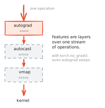
Figure 22. every feature watches the same stream of operations. a context manager puts one layer to sleep.
PyTorch's features combine cleanly because each one is a layer in the dispatcher, watching the same stream of operations:
>>> with torch.no_grad():
...     z = a * 2
>>> z.grad_fn is None              # nothing was recorded
True
no_grad edited no function. It set a flag that sends operations
past the autograd layer, so nothing gets recorded. Mixed precision,
tracing and vmap work the same way, and that is why they can be
combined without knowing about each other. Part 5 opens the
machinery under the flag.
6. Every operation pays a fixed cost first
full story: Part 7, The Compiler
Half a microsecond of crossing and routing before any math, on
every single operation. That was the measurement on the boundary
floor. Applied honestly, this one number explains why
torch.compile exists, why fused optimizers exist, and why the
first question about any slow model is: is it limited by compute,
or by the cost of issuing many small operations?
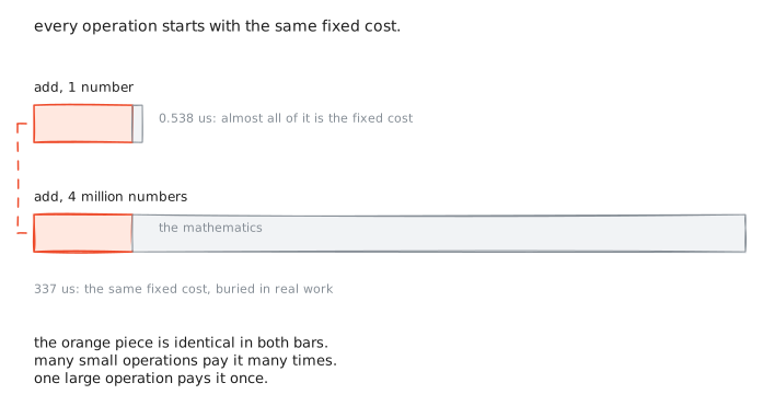
Interactive 3. the same add at twelve measured sizes. the dots are measured on the author's machine; plant your flag before the curve appears. This is a live instrument in the original post; the still drawing stands in here.
7. Memory, not speed, is what kills training runs
full story: Part 4, Seeing PyTorch
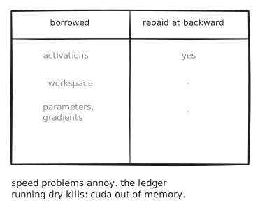
Figure 23. the forward pass borrows memory. backward repays it. running out is the most common way a training run dies.
A slow program still finishes. A program that runs out of GPU
memory dies with CUDA out of memory, and that is the most common
death in all of PyTorch. The forward pass saves values for
backward (the turn, above). The allocator keeps and reuses blocks.
Between them they decide how large a model you can train. This
series treats memory as a first-class subject in Part 4.
8. Python is why it won, and what it costs
full story: Part 7, The Compiler
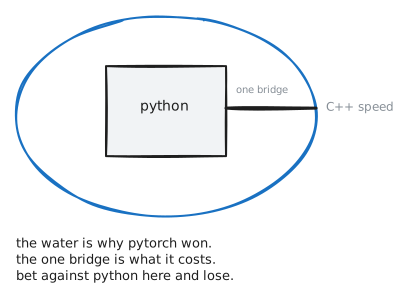
Figure 24. the protection and the price are the same picture: everything must cross one bridge.
PyTorch won because you write it in ordinary Python, with ordinary debuggers and print statements. The price is the border cost from Idea 6, paid on every operation. The history of the framework is a sequence of attempts to keep the first while reducing the second. TorchScript tried to replace Python with its own language; it is now in maintenance mode [4]. The current compiler watches your Python run and translates what it can, and it is winning. The pattern to remember: inside PyTorch, betting against Python has always lost.
9. Forward decides what backward must do
full story: Part 9, Distributed
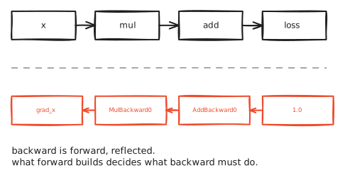
Figure 25. backward is the reflection of the graph forward wrote.
Backward can only walk what forward wrote. On one machine this sounds like a detail. At scale it becomes the law of the land: in distributed training, the way a tensor is split across GPUs in the forward pass decides which GPUs must exchange data in the backward pass. One idea, from a laptop to a cluster. It is the spine of Part 9.
10. Shared bytes plus in-place writes cause the hardest problems
full story: Part 2, Autograd
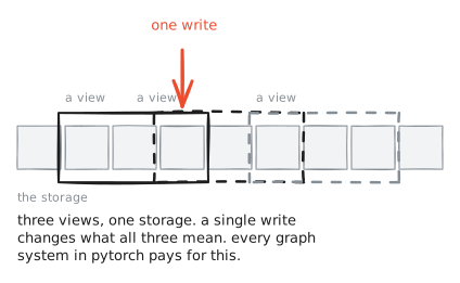
Figure 26. three windows, one storage, one write. every system that records or rewrites programs must handle this.
Idea 1 lets many tensors read the same bytes. Idea 2 lets you change those bytes in place. Combine them: one write can change the meaning of several tensors at once, and any system that records programs (autograd, the compiler, export) must notice and stay correct. When a corner of PyTorch looks strangely complicated, ask what shared bytes plus an in-place write would do to it. That is usually the answer.
11. The code keeps its history
full story: Part 5, The Machinery
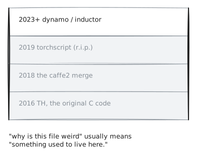
Figure 27. four systems, four eras, one repository. older layers still show through.
The repository holds the remains of every era: the original C code from 2016, the Caffe2 merge of 2018, TorchScript from 2019, the compiler district growing since 2023. When a file looks strange, the explanation is usually historical: something older lived there first. Part 5 tells this history where it explains the present.
12. Floating point is a contract; read it
full story: Part 4, Seeing PyTorch
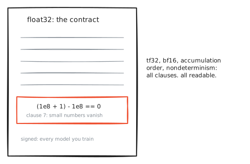
Figure 28. the terms are public. every training run signs them.
>>> t = torch.tensor(1e8)
>>> ((t + 1) - t).item()
0.0
A float32 number has about 7 decimal digits of precision, so adding 1 to one hundred million changes nothing [5]. This is not a bug; it is the number format doing what it promises. Add the faster, less precise formats used in training, plus the fact that some GPU kernels sum in different orders on different runs, and "why did my loss change between runs" becomes a question with exact answers. Part 4 reads this contract clause by clause.
How this series draws
Every still figure you just saw is a real Excalidraw scene, and the scene files ship with the series; you can open any drawing and edit it. The four instruments you can operate follow the same language, and every number inside them comes from the proof scripts. All of them speak one visual language, so that by Part 2 you read them without thinking:
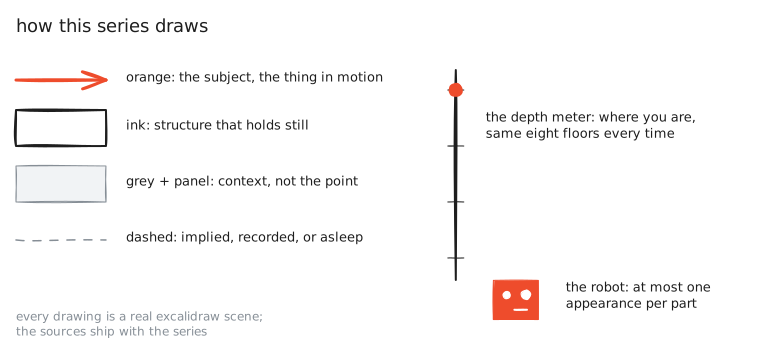
Figure 29. the whole notation on one sheet. learn it once; it holds for the entire series.
Orange always marks the subject: the one thing moving. Ink is structure. Grey is context. Dashed means recorded, implied, or asleep. The depth meter marks the floor. And the robot appears at most once per part, because a mascot that is everywhere stops being funny.
How to read this
Twelve parts. Each is one long page like this one. And the series has one quiet goal behind every part: by the end, you should know the machine well enough to build a small PyTorch yourself. Every drawing that shows a mechanism, every formula next to a figure, and every proof script is a piece of that.
| Part | What is behind the door |
|---|---|
| 0. The Map | you are here |
| 1. Tensor | storage, strides, views, data types, broadcasting |
| 2. Autograd | the graph, in-place writes, checkpointing, double backward |
| 3. Daily PyTorch | nn, optim, data loading, mixed precision, seen from inside |
| 4. Seeing PyTorch | the profiler, memory, floating point, honest measurement |
| 5. The Machinery | the dispatcher, aten, torchgen, the history |
| 6. Extending PyTorch | subclasses, custom operations, new backends |
| 7. The Compiler | dynamo, aot autograd, inductor, dynamic shapes |
| 8. Kernels & Hardware | the gpu model, triton, cutlass, what fast means |
| 9. Distributed | collectives, ddp, fsdp, dtensor, parallel training |
| 10. Ship It | export, quantization, executorch, the ecosystem |
| 11. Working on PyTorch | the contributor's field guide |
You do not have to read front to back. Three reading lines run through the parts, like lines through stations:
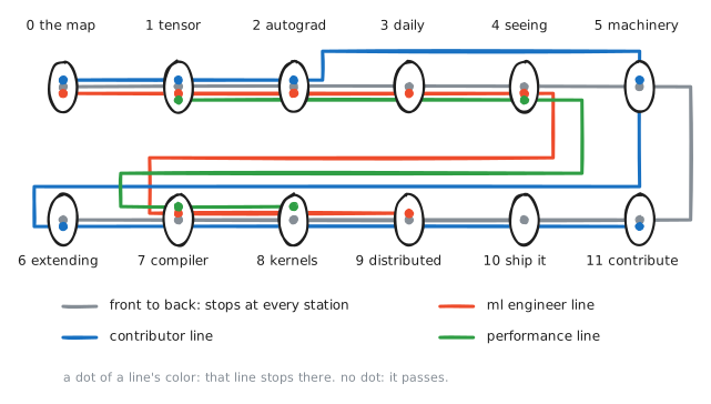
Interactive 4. pick a line. grey is front to back and stops everywhere; orange fits most readers; green chases speed; blue is the one for a new contributor. a dot means the line stops there. This is a live instrument in the original post; the still drawing stands in here.
Every chapter inside every part follows the same seven steps, so the rhythm becomes familiar fast:
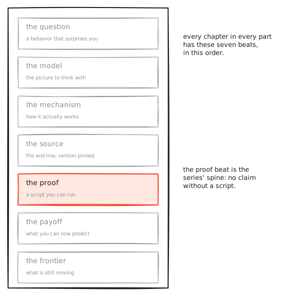
Figure 30. the seven steps of every chapter. the proof step is the spine: no claim without a script.
And the method, stated plainly, because you should know what you are trusting. Every mechanism claim is checked against the source code or shown by a script before it is published. The scripts are linked in place and pinned to one torch version. When PyTorch moves and a claim goes stale, the chapter is corrected and the correction is noted on the page. A series about internals that cannot admit drift would be wrong within a year.
What you can now say
Test yourself against this list. After one reading you should be able to say, in your own words:
- what
type(torch.randn)returns, and where the compiled body actually lives on your disk - what the dispatcher is, and how
no_gradstops autograd without editing any function - what a kernel is, and what decides which one runs
- why the CPU and the GPU run on two clocks, and why that makes simple timing code lie
- what the graph is, who writes it, and why backward can never do anything forward did not write down
- and the twelve ideas, each in one sentence
If one of these is fuzzy, return to its floor; each one is only a minute long. That is what this page is for.
Try it yourself
The five proof scripts are the exercises. For each one: predict the output first, then run it, then explain the difference.
- p0_the_library.py: how big are the compiled libraries in your own torch install?
- p1_graph_chain.py: what graph remains after a two-layer model runs?
- p2_dispatch_cost.py: what is the fixed cost per operation on your machine?
- p3_two_timelines.py: how long is your GPU still working after Python is done asking?
- p4_micro_proofs.py: the twelve ideas, compressed into five small experiments.
Pick a door
Part 1 is the tensor. It opens with the puzzle from Idea 1, and now you have seen the error with your own eyes:
>>> v.t().view(-1)
RuntimeError: view size is not compatible with input tensor's
size and stride ...
>>> v.t().reshape(-1)   # this one works. why?
tensor([0., 3., 1., 4., 2., 5.])
Same tensor. Same request. One line refuses, the other quietly copies the data. The difference between those two lines is the whole first part of this series.
See you on the next floor down.
References
[1] Khalilli, five proof scripts, measured on an Apple M3 Max, torch 2.11.0, CPU and Apple GPU, 2026. Linked in place above; rerun them to check me.
[2] PyTorch source, native_functions.yaml, pinned to the v2.11.0 tag. https://github.com/pytorch/pytorch/blob/v2.11.0/aten/src/ATen/native/native_functions.yaml
[3] PyTorch source, derivatives.yaml, pinned to the v2.11.0 tag. https://github.com/pytorch/pytorch/blob/v2.11.0/tools/autograd/derivatives.yaml
[4] PyTorch documentation, TorchScript, which states it is in maintenance mode. https://docs.pytorch.org/docs/stable/jit.html
[5] IEEE, 754 single precision: 24 binary digits of precision, about 7 decimal digits.
Three good things to read after this page: Edward Yang's PyTorch internals talk, which maps the C++ side in depth; the PyTorch Developer Podcast, short episodes by the same author; and the repository's own CONTRIBUTING.md, which describes the folder layout in the maintainers' words.