---
license: apache-2.0
library_name: pytorch
pipeline_tag: graph-ml
language:
- en
tags:
- graph-neural-network
- gnn
- meshgraphnet
- film
- surrogate-model
- scientific-machine-learning
- physics-ml
- heat-transfer
- casting
- metal-casting
- foundry
- solidification
- finite-element
- fenicsx
- pytorch-geometric
- scikit-learn
---
# Casting solidification GNN (v5.1)
A surrogate model for the solidification of metal castings in a sand mold. It takes a
tetrahedral mesh of a casting together with the alloy and mold properties, and predicts the
time at which every mesh node solidifies. The nodes that solidify last are the hot spots, where
feeding problems and shrinkage defects usually start.
A transient finite-element solve of the same field takes minutes to hours. The model returns it
in seconds, which makes it useful for screening design variants before a full simulation. It
does not replace a calibrated process simulation or physical validation, and a hot spot is a
shrinkage-risk indicator, not a porosity label.
To look at predictions without installing anything, open the [demo Space](https://huggingface.co/spaces/eugenmik/castsolid-gnn-demo): it shows
four parts in two alloys in 3D, with the hot spots and a shrinkage screening.
A predicted field played back over time. Solidified material turns translucent while the
remaining liquid contracts toward the hot spot.
| | |
|---|---|
| Version | v5.1, frozen on 31 July 2026 |
| Task | Per-node regression on a tetrahedral mesh (graph ML) |
| Input | Tetrahedral mesh in mm (gmsh 2.2 format) with the cooling surface tagged; alloy `EN-GJS-400-15` or `G20Mn5`, or a custom property set; green-sand mold |
| Output | Solidification time in seconds for every mesh node |
| Architecture | 12-block MeshGraphNet-style GNN with FiLM conditioning, combined with two gradient-boosted heads |
| Parameters | about 1.85 M (GNN) plus two `HistGradientBoostingRegressor` heads |
| Training data | FEniCSx enthalpy-method conduction simulations: about 9.7k primitive cases, 4.7k multi-alloy cases, 500 real-part cases |
| License | Apache-2.0 for code and weights |
| Demo | [castsolid-gnn-demo](https://huggingface.co/spaces/eugenmik/castsolid-gnn-demo): precomputed predictions in 3D, no installation |
| Code | [github.com/eugenmik/castsolid-gnn](https://github.com/eugenmik/castsolid-gnn): loading, inference, and the STEP-to-result pipeline |
| Author | Eugen Miknevic, independent foundry engineer |
## Contents
- [Input and output](#input-and-output)
- [How to use](#how-to-use)
- [Model architecture](#model-architecture)
- [Files](#files)
- [Training data](#training-data)
- [Training procedure](#training-procedure)
- [Evaluation](#evaluation)
- [Intended use and limitations](#intended-use-and-limitations)
- [Reproducibility](#reproducibility)
- [License and citation](#license-and-citation)
## Input and output
The model reads one casting at a time.
The mesh is a tetrahedral volume mesh in millimetres, in gmsh 2.2 ASCII format (`.msh`). Surface
triangles that cool into the mold belong to a physical group named `Cooling`; in this release
that is the whole outer surface. The model was trained on meshes of roughly 7,500 to 10,000
nodes, and that is the density it should be given. It does not use node numbering or absolute
coordinates: node inputs are distances, flags and volume-type quantities in millimetres, and
edges carry only relative displacements between neighbouring nodes.
Eight numbers describe the alloy and the mold: thermal conductivity, density, specific heat,
latent heat, liquidus, solidus, pouring temperature and mold effusivity. The code ships two
tabulated alloys, `EN-GJS-400-15` (ductile iron, the default) and `G20Mn5` (cast steel), and one
mold, green sand. You can also pass your own eight values.
The output is one number per node: the time in seconds at which that node cools through the
solidus. The maximum over all nodes is the total solidification time, and the 10% of nodes with
the largest times are the hot spots.
## How to use
This repository holds the weights and this card. The code that loads and runs them is on
[GitHub](https://github.com/eugenmik/castsolid-gnn):
```bash
git clone https://github.com/eugenmik/castsolid-gnn
cd castsolid-gnn
python -m venv .venv && source .venv/bin/activate
pip install "torch==2.3.0" --index-url https://download.pytorch.org/whl/cpu
pip install torch-cluster -f https://data.pyg.org/whl/torch-2.3.0+cpu.html
pip install -r requirements.txt
```
Python 3.11 is recommended. For a GPU, replace `cpu` with your CUDA tag (for example `cu121`)
in both URLs. Then, from the repository root:
```python
from src.model_api import CastSolidModel
model = CastSolidModel.from_pretrained() # downloads this repository's files once
t = model.predict("part.msh") # EN-GJS-400-15 in green sand
t_steel = model.predict("part.msh", alloy="G20Mn5")
t.max() # total solidification time, s
hot = CastSolidModel.hotspots(t) # boolean mask, top 10% of nodes
```
`from_pretrained()` fetches `config.json` and the files it lists into the local Hugging Face
cache, pinned to the `v5.1` tag; later calls run offline. `predict` returns a NumPy array in the
node order of the `.msh` file. To use another alloy, pass `props_json="my_alloy.json"` with
exactly these keys (SI units, temperatures in °C; 1018 is the green-sand effusivity):
```json
{"k": 32.9, "rho": 6800.0, "cp": 515.0, "L_kJ_kg": 220.0,
"TL": 1160.0, "TS": 1120.0, "Tpour": 1260.0, "mold_effusivity": 1018.0}
```
To start from a STEP file instead of a mesh, run `python -m src.predict_casting part.step` in
the GitHub repository. It heals the CAD, builds a mesh at the right density, runs the model and
writes the result for ParaView.
## Model architecture
The model is a hybrid of three trained parts. The GNN predicts the spatial shape of the field;
two gradient-boosted heads predict its overall level and its spread; a fixed recomposition step
combines them. The GNN alone is less reliable about absolute magnitude, which depends strongly
on alloy and part size. On the original benchmark of held-out geometry families, adding the
heads brought nodal MAE down from 5.77 s to 4.26 s.
```mermaid
flowchart LR
M[Tetrahedral mesh] --> F[15 node features
+ union graph]
P[Alloy + mold
properties] --> G[5-value conditioning vector]
P --> D
F --> N[12-block GNN
field shape]
G --> N
F --> D[Part descriptors]
D --> T[GBM total head]
D --> S[GBM spread head]
N --> R[Soft-anchor
recomposition]
T --> R
S --> R
R --> O[Time per node, s]
```
### Graph network
Nodes are mesh vertices. Edges are the union of the tetrahedral mesh edges and the 16 nearest
neighbours of each node. Each edge carries its displacement vector, its length and a flag that
says whether it is a mesh edge.
Each node gets 15 features computed from the mesh and its surface tags:
- geodesic distance through the mesh to the nearest cooling surface and to the nearest
adiabatic surface, plus straight-line distance to the surface and to adiabatic faces;
- cooling, adiabatic and interior flags;
- part volume, surface area and the fraction of surface that cools;
- local modulus, the volume-to-surface ratio inside geodesic balls of 5, 15 and 40 mm, which is
a local version of Chvorinov's modulus;
- two boundary-condition channels: the mold effusivity on surface nodes (zero inside the
part), and a boundary heat-input channel, which is zero because a sand-mold surface adds no
heat.
The alloy and mold enter as five dimensionless numbers: Stefan number, normalized freezing
range, thermal diffusivity ratio, normalized superheat and normalized mold effusivity. They
condition every processor block through FiLM (`h ← h·(1+γ(g)) + β(g)`).
The network follows the encode-process-decode design of
[MeshGraphNets](https://arxiv.org/abs/2010.03409). MLP encoders embed nodes and edges, 12
message-passing blocks (hidden width 128, residual connections, LayerNorm, mean aggregation)
process them, and a two-head decoder predicts the per-node deviation and a graph-level scale
separately. The training target is the standardized `log1p` of the solidification time.
### Gradient-boosted heads
Both heads are scikit-learn `HistGradientBoostingRegressor` models with one row per part: the
alloy properties, the part's volume-to-area ratio, the mold effusivity, and boundary-condition
descriptors that are fixed to the plain sand mold in this release. The total head (16 inputs)
predicts `log1p` of the total solidification time. The spread head (17 inputs, absolute-error
loss) predicts `log1p` of the standard deviation of the nodal field.
### Soft-anchor recomposition
The GNN field is scaled, shifted and clipped at zero,
```
pred(a, m) = max(0, a · (gnn − mean(gnn)) + m)
```
with `(a, m)` chosen to minimize
```
J = w_total · ((q99.5(pred) − T_total) / T_total)² + w_std · ((std(pred) − S) / S)²
```
where `T_total` and `S` come from the two heads, `w_total = 1` and `w_std = 4`. When both
targets can be met exactly, this equals the closed-form affine solve. When clipping makes that
impossible, the total anchor may move by a few percent so the spread stays close. The post-clip
spread is not monotone in `a`, so the solver brackets the smallest root explicitly.
## Files
| File | Size | Content |
|---|---:|---|
| `config.json` | 1 KB | Model version, file list, architecture summary, recomposition weights and input description |
| `gnn_v5.1.safetensors` | 7.4 MB | GNN weights, feature and target normalization, and the architecture config (in the safetensors metadata) |
| `gbm_total_v3.skops` | 0.6 MB | Total-time head |
| `gbm_std_v2.skops` | 0.8 MB | Spread head |
| `ood_ranges.json` | <1 KB | Training envelope (part volume, size, distance to cooling) used for out-of-distribution warnings |
None of the weight files can execute code when loaded. The GNN is stored as
[safetensors](https://github.com/huggingface/safetensors) and the heads as
[skops](https://skops.readthedocs.io/). Before it opens a skops file, the loader on GitHub checks
every type the file names against an allowlist of scikit-learn and NumPy types. Training code is
not published.
## Training data
Every reference field was computed with [FEniCSx](https://fenicsproject.org/) (dolfinx) using an
enthalpy-method model of transient heat conduction with latent heat. There is no mold filling,
flow, gas or stress in it.
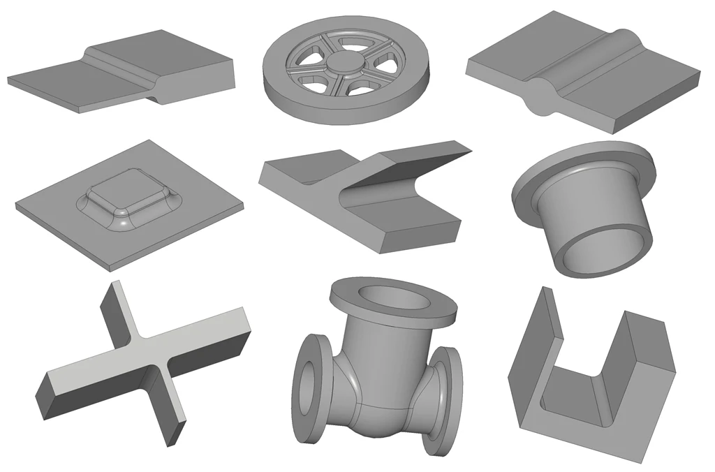
Some of the primitive geometry families from the first training regime.
| Set | Cases | Content |
|---|---:|---|
| Primitives (original regime) | 9,710 | 42 parametric geometry families, a single alloy, sand mold, different assignments of cooling and adiabatic faces |
| Multi-alloy (v4) | 4,727 | Realistic thick-walled castings in 12 named iron and steel grades plus sampled synthetic alloys, under several boundary-condition regimes |
| Real parts (E) | 500 | Prepared production geometries with varied boundary conditions |

Training meshes carry three physical groups: Volume, Cooling (mold contact) and
Adiabatic.
Training meshes have roughly 7,500 to 10,000 nodes. The target at each node is the time its
temperature drops through the solidus. Material properties come from handbook data. The raw
simulation corpus (about 100 GB) is not distributed.
One data issue shaped this project more than any model choice. The solver stored temperatures
in dolfinx degree-of-freedom order, while coordinates and geometric features were in gmsh node
order, so about 60% of the nodal targets were silently attached to the wrong positions. Every
early model failure traced back to it. The training set was rebuilt with a recovered
permutation between the two orderings. If you train on solver output, check node identity across
every solver and mesh interface before tuning a model.
## Training procedure
v5.1 came out of a chain of fine-tunes, not a single training run.
1. SP1 trained a 12-block two-head GNN from scratch on the primitive set, with the union graph,
local-modulus features and a loss on both nodal and total time.
2. FT2b fine-tuned it on the multi-alloy set. The FiLM layers started at zero, so training began
from exactly the SP1 function.
3. A follow-up pass re-encoded one sparse boundary input as a field diffused along the mesh,
because the network had learned to suppress it, and picked the checkpoint on gate metrics
instead of validation loss alone.
4. FT3 fine-tuned on real production geometries (set E) with the normalization statistics
frozen. Its epoch-21 checkpoint is the v5.1 GNN.
5. The total head (v3), the absolute-error spread head (v2) and the recomposition weights were
selected on held-out real-part validation rows.
Training ran on one RTX 3060 (12 GB) with batch size 2, at 15 to 20 minutes per epoch. To be
promoted, v5.1 had to pass four gates on held-out data: two gold-standard real parts, 24
held-out real parts, an extrapolation split and a check against collapsed field variance.
## Evaluation
Do not compare numbers across regimes. Total times in the primitive regime are tens of seconds;
on real geometry they run to hundreds or thousands.
| Evaluation | n | Nodal MAE | Hot-spot overlap | What it shows |
|---|---:|---:|---:|---|
| Held-out primitive geometry families | family split | 4.26 s | 0.917 | Generalization to unseen synthetic shape families in the original regime |
| Unseen real single-body castings | 6 | 80.3 s median | 0.738 median | Generalization to new real geometry, scored against a FEniCSx reference on the same mesh |
Hot-spot overlap compares the 10% of nodes that solidify last in the prediction with the same
set in the reference. 1.0 means the two sets are identical.
One of the six real parts reached a hot-spot overlap of only 0.035, so the median says nothing
certain about any one part.
> **Important.** The training data and the real-geometry references come from the same FEniCSx
> heat-transfer model, the same material database and the same boundary assumptions. These
> numbers measure how well the surrogate carries over to new geometry. They are not evidence of
> physical accuracy against instrumented castings.
## Intended use and limitations
Good uses:
- comparing early casting concepts;
- finding candidate last-to-solidify regions;
- deciding which designs need a full process simulation;
- early quoting and design discussions, as long as the limitations stay visible.
Out of scope:
- final process sign-off or contractual acceptance;
- guaranteed defect or porosity prediction;
- mold filling, flow, gas, stress or distortion;
- unattended decisions on geometry outside the training envelope;
- safety-critical decisions without an independent engineering review.
Known limitations:
1. The physics is pure conduction with latent heat, and the reference solver shares the model's
property and boundary assumptions.
2. This release covers one setup: a single casting whose whole outer surface cools into a
green-sand mold, in `EN-GJS-400-15`, `G20Mn5` or a custom property set.
3. Meshes much coarser or finer than the training density (about 7,500 to 10,000 nodes) are
outside what the model has seen. At that density, large thin-walled parts can be
under-resolved.
4. The training envelope in `ood_ranges.json` only covers part size and distance to
cooling. It is not a calibrated uncertainty estimate.
Treat each prediction as a screening hypothesis: where should an engineer look first, and is
the concept ready for a full simulation? Keep the mesh, the inputs and the model version with
every result, and send high-consequence cases to a calibrated simulation and a physical review.
## Reproducibility
The published files were converted from the internal training checkpoints and checked against
them:
| Release file | Internal artifact | Check |
|---|---|---|
| `gnn_v5.1.safetensors` | `ckpt_ep021.pt` (FT3, epoch 21) | Every tensor bit-identical; same config and normalization |
| `gbm_total_v3.skops` | `hgb_v3.joblib` | Identical predictions on 10,002 probe rows spanning each feature's training split range |
| `gbm_std_v2.skops` | `hgb_std_v2.joblib` | Identical predictions on 10,002 probe rows spanning each feature's training split range |
The published inference code was also run side by side with the internal pipeline on five
production parts (two of them with both alloys), plus a fixed-size mesh with a custom property
set: every output field matched exactly. The heads were trained with scikit-learn 1.5.2, and other versions may refuse to load them or change
their output. Other versions used: Python 3.11, PyTorch 2.3.0, PyTorch Geometric 2.7.0,
NumPy 2.x.
## License and citation
Code and weights are released under the [Apache License 2.0](LICENSE). The tables in
`data/properties/` of the GitHub repository are modelling inputs, not certified material
specifications.
```bibtex
@software{miknevic_casting_gnn_2026,
author = {Miknevic, Eugen},
title = {Casting Solidification GNN: a graph neural network surrogate for
rapid solidification screening of metal castings},
version = {5.1},
year = {2026},
url = {https://huggingface.co/eugenmik/castsolid-gnn}
}
```
Contact: Eugen Miknevic, eugenmiknevic@gmail.com. If you have failure cases, questions or
measured data from real castings, please post them in the
[Community tab](https://huggingface.co/eugenmik/castsolid-gnn/discussions).