artifacts/bp_gaussian_tutorial.py

import marimo

__generated_with = "0.23.14"
app = marimo.App(width="medium")


@app.cell
def _():
    import marimo as mo

    return (mo,)


@app.cell
def _(mo):
    mo.md(r"""
    # When belief propagation becomes Gaussian

    ![Across chain, tree, and loopy graphs, KL to a fitted Gaussian falls below 0.02 before distance three.](https://raw.githubusercontent.com/MachineLearning-Nerd/icml26-repro-FaGn04tvzq-bp-gaussian/master/reports/bp-gaussian/images/headline_topologies.png)

    This tutorial explains the central claim of
    [arXiv:2601.21935](https://arxiv.org/abs/2601.21935) from already-captured
    evidence. It does **not** rerun the formal experiments.

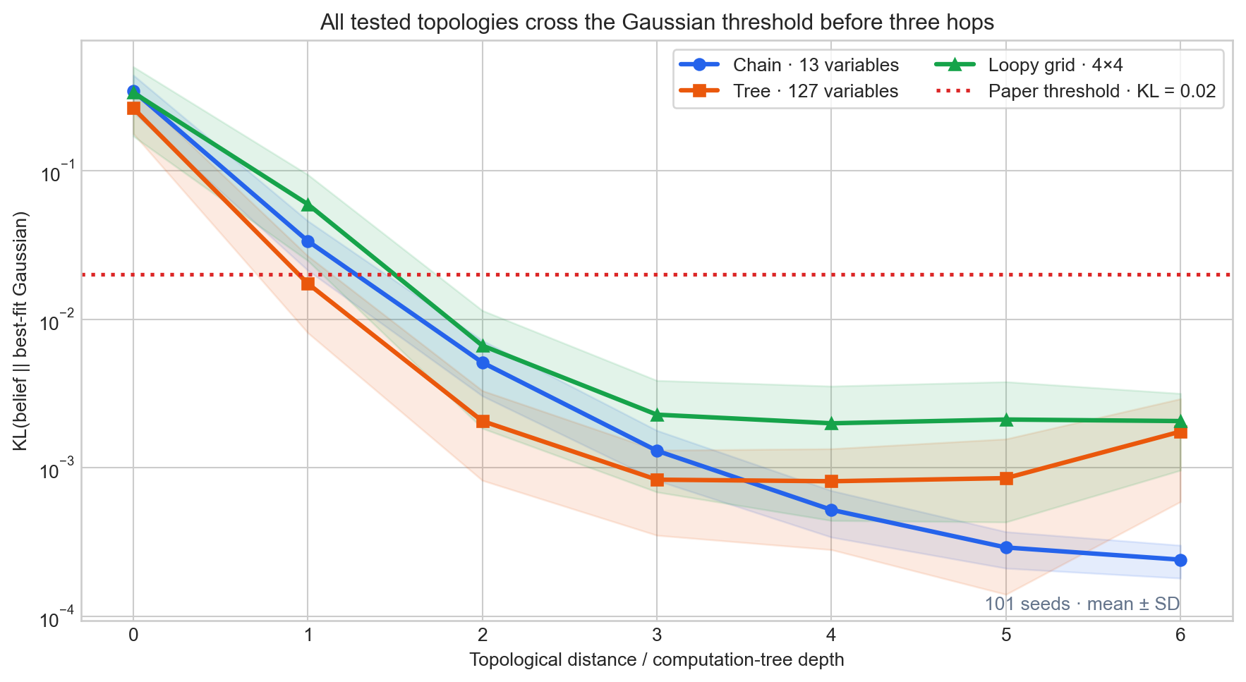
    The idea is simple: a pairwise BP update repeatedly convolves probability
    distributions along a path. Convolution suppresses non-Gaussian structure,
    so beliefs can become approximately Gaussian even when the original priors
    are not. Across 101 seeds, the chain, 127-node tree, and loopy grid were all
    below the paper's `KL < 0.02` threshold before three hops.
    """)
    return


@app.cell
def _():
    evidence = {
        "Chain": [0.34412, 0.03361, 0.00511, 0.00130, 0.00052, 0.00029, 0.00024],
        "Tree": [0.26382, 0.01738, 0.00206, 0.00083, 0.00081, 0.00085, 0.00175],
        "Loopy grid": [0.33620, 0.05946, 0.00664, 0.002275, 0.00199, 0.00211, 0.00206],
    }
    return (evidence,)


@app.cell
def _(mo):
    threshold = mo.ui.slider(
        start=0.001,
        stop=0.05,
        step=0.001,
        value=0.02,
        label="Gaussian KL threshold",
        show_value=True,
    )
    threshold
    return (threshold,)


@app.cell
def _(evidence, mo, threshold):
    rows = []
    for topology, values in evidence.items():
        crossings = [distance for distance, value in enumerate(values) if value < threshold.value]
        first = crossings[0] if crossings else "not reached"
        rows.append(f"| {topology} | {values[0]:.5f} | {values[3]:.6f} | {first} |")
    mo.md(
        f"""
        ## Explore the threshold

        | Topology | KL at prior | KL at distance 3 | First distance below {threshold.value:.3f} |
        |---|---:|---:|---:|
        {chr(10).join(rows)}

        This slider changes only the interpretation of embedded evidence. It
        does not recompute BP or modify the registered result.
        """
    )
    return


@app.cell
def _(mo):
    mo.md(r"""
    ## Two controls identify the mechanism

    ![The repeated-convolution chain Gaussianizes; disabling convolution leaves KL constant.](https://raw.githubusercontent.com/MachineLearning-Nerd/icml26-repro-FaGn04tvzq-bp-gaussian/master/reports/bp-gaussian/images/mechanism_controls.png)

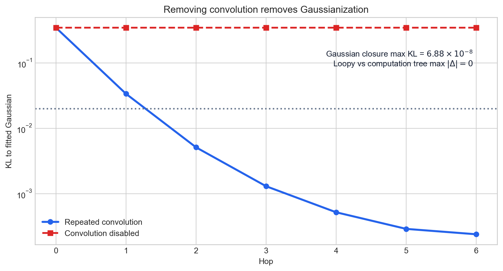    Disabling convolution removes the KL decay. Convolving Gaussian inputs
    stays Gaussian to a maximum numerical residual of `6.877×10⁻⁸`, and the
    direct loopy message equals its depth-four computation-tree counterpart
    exactly. These checks make the topology curves causal evidence rather than
    a visual coincidence.

    A star supplies the complementary negative control: its center gets more
    neighbors but no path depth. Mean center KL rises from `0.06618` at degree
    2 to `0.18719` at degree 10, with positive slopes in all 31 paired seeds.
    """)
    return


@app.cell
def _(mo):
    mo.md(r"""
    ## The analytic boundary

    Solving the Appendix-D equation gives `R*=6.0168484964`, within `0.016848`
    of the paper's `R≈6` boundary. A separate finite-grid Figure-4c sweep did
    not show its reported low-KL transition, so the report keeps those two
    pieces of evidence separate: **analytic alignment, empirical-sweep
    divergence in this implementation**.

    ## Real Middlebury Cones

    ![Official Cones accuracy and spatial KL result.](https://raw.githubusercontent.com/MachineLearning-Nerd/icml26-repro-FaGn04tvzq-bp-gaussian/master/reports/bp-gaussian/images/stereo_real.png)

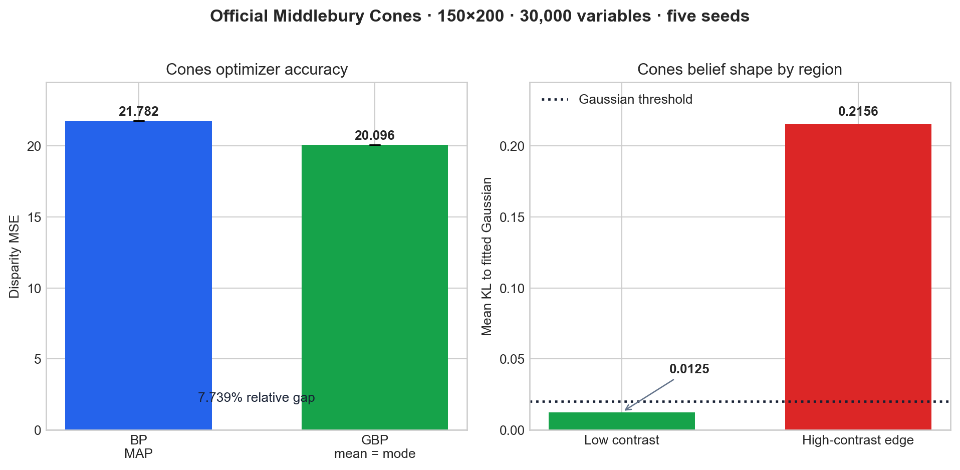    The registered real-data audit uses 150×200 pixels (30,000 variables), 28
    disparity labels, official Cones imagery, and five seeds. BP MAP MSE is
    `21.781727 ± 0.003305`; GBP is `20.096043 ± 0.000000`, a `7.739%` gap.
    Low-contrast mean KL is `0.012508`, while edge mean KL is `0.215593`.
    """)
    return


@app.cell
def _(mo):
    mo.md(r"""
    ## Six claim groups, one transparent assessment

    | Claim | Observed evidence | Assessment |
    |---|---|---|
    | Chain convergence | Hop-3 KL `0.001303` over 101 seeds | Aligned |
    | Tree convergence | Hop-3 KL `0.000826`; 127 nodes, 64 leaf priors | Aligned |
    | Loopy computation tree | Hop-3 KL `0.002275`; exact message difference `0` | Aligned |
    | Exclusion boundary | Analytic `R*=6.016848`; finite-grid sweep divergent | Analytically aligned |
    | Degree control | `31/31` positive paired slopes | Aligned |
    | Real stereo | `7.739%` MSE gap; low-contrast/edge KL split | Aligned under registered criterion |

    The formal CPU command is shown for provenance; running it downloads Cones
    and can take several minutes. The evidence above is embedded so Molab
    readers do not need to rerun it.

    ```bash
    python -m venv .venv && . .venv/bin/activate && python -m pip install --disable-pip-version-check numpy==2.3.2 && python repro/src/verify_bp.py
    ```

    Read the [full illustrated report](https://github.com/MachineLearning-Nerd/icml26-repro-FaGn04tvzq-bp-gaussian/blob/master/reports/bp-gaussian/report.md)
    for implementation details, substitutions, and immutable experiment links.
    """)
    return


if __name__ == "__main__":
    app.run()