# Working with large data using Datashader
The various plotting-library backends supported by HoloViews, such as Matplotlib, Bokeh, and Plotly, each have limitations on the amount of data that is practical to work with. Bokeh and Plotly in particular mirror your data directly into an HTML page viewable in your browser, which can cause problems when data sizes approach the limited memory available for each web page in current browsers.
Luckily, a visualization of even the largest dataset will be constrained by the resolution of your display device, and so one approach to handling such data is to pre-render or rasterize the data into a fixed-size array or image *before* sending it to the backend plotting library and thus to your local web browser. The [Datashader](https://github.com/bokeh/datashader) library provides a high-performance big-data server-side rasterization pipeline that works seamlessly with HoloViews to support datasets that are orders of magnitude larger than those supported natively by the plotting-library backends, including millions or billions of points even on ordinary laptops.
Here, we will see how and when to use Datashader with HoloViews Elements and Containers. For simplicity in this discussion we'll focus on simple synthetic datasets, but [Datashader's examples](http://datashader.org/topics) include a wide variety of real datasets that give a much better idea of the power of using Datashader with HoloViews, and [HoloViz.org](http://holoviz.org) shows how to install and work with HoloViews and Datashader together.
```python
import datashader as ds
import numpy as np
import holoviews as hv
import pandas as pd
import numpy as np
from holoviews import opts
from holoviews.operation.datashader import datashade, rasterize, shade, dynspread, spread
from holoviews.operation.resample import ResampleOperation2D
from holoviews.operation import decimate
hv.extension('bokeh','matplotlib', width=100)
# Default values suitable for this notebook
decimate.max_samples=1000
dynspread.max_px=20
dynspread.threshold=0.5
ResampleOperation2D.width=500
ResampleOperation2D.height=500
def random_walk(n, f=5000):
"""Random walk in a 2D space, smoothed with a filter of length f"""
xs = np.convolve(np.random.normal(0, 0.1, size=n), np.ones(f)/f).cumsum()
ys = np.convolve(np.random.normal(0, 0.1, size=n), np.ones(f)/f).cumsum()
xs += 0.1*np.sin(0.1*np.array(range(n-1+f))) # add wobble on x axis
xs += np.random.normal(0, 0.005, size=n-1+f) # add measurement noise
ys += np.random.normal(0, 0.005, size=n-1+f)
return np.column_stack([xs, ys])
def random_cov():
"""Random covariance for use in generating 2D Gaussian distributions"""
A = np.random.randn(2,2)
return np.dot(A, A.T)
def time_series(T = 1, N = 100, mu = 0.1, sigma = 0.1, S0 = 20):
"""Parameterized noisy time series"""
dt = float(T)/N
t = np.linspace(0, T, N)
W = np.random.standard_normal(size = N)
W = np.cumsum(W)*np.sqrt(dt) # standard brownian motion
X = (mu-0.5*sigma**2)*t + sigma*W
S = S0*np.exp(X) # geometric brownian motion
return S
```
This notebook makes use of dynamic updates, which require a running a live Jupyter or Bokeh server.
When viewed statically, the plots will not update fully when you zoom and pan.
# Principles of datashading
Because HoloViews elements are fundamentally data containers, not visualizations, you can very quickly declare elements such as ``Points`` or ``Path`` containing datasets that may be as large as the full memory available on your machine (or even larger if using Dask dataframes). So even for very large datasets, you can easily specify a data structure that you can work with for making selections, sampling, aggregations, and so on. However, as soon as you try to visualize it directly with either the Matplotlib, Plotly, or Bokeh plotting extensions, the rendering process may be prohibitively expensive.
Let's start with a simple example that's easy to visualize in any plotting library:
```python
np.random.seed(1)
points = hv.Points(np.random.multivariate_normal((0,0), [[0.1, 0.1], [0.1, 1.0]], (1000,)),label="Points")
paths = hv.Path([random_walk(2000,30)], kdims=["u","v"], label="Paths")
points + paths
```
These browser-based plots are fully interactive, as you can see if you select the Wheel Zoom or Box Zoom tools and use your scroll wheel or click and drag.
Because all of the data in these plots gets transferred directly into the web browser, the interactive functionality will be available even on a static export of this figure as a web page. Note that even though the visualization above is not computationally expensive, even with just 1000 points as in the scatterplot above, the plot already suffers from [overplotting](https://anaconda.org/jbednar/plotting_pitfalls), with later points obscuring previously plotted points.
With much larger datasets, these issues will quickly make it impossible to see the true structure of the data. We can easily declare 50X or 1000X larger versions of the same plots above, but if we tried to visualize them directly they would be unusably slow even if the browser did not crash:
```python
np.random.seed(1)
points = hv.Points(np.random.multivariate_normal((0,0), [[0.1, 0.1], [0.1, 1.0]], (1000000,)),label="Points")
paths = hv.Path([0.15*random_walk(100000) for i in range(10)], kdims=["u","v"], label="Paths")
#points + paths ## Danger! Browsers can't handle 1 million points!
```
Luckily, HoloViews Elements are just containers for data and associated metadata, not plots, so HoloViews can generate entirely different types of visualizations from the same data structure when appropriate. For instance, in the plot on the left below you can see the result of applying a `decimate()` operation acting on the `points` object, which will automatically downsample this million-point dataset to at most 1000 points at any time as you zoom in or out:
```python
decimate( points).relabel("Decimated Points") + \
rasterize(points).relabel("Rasterized Points").opts(colorbar=True, width=350) + \
rasterize(paths ).relabel("Rasterized Paths")
```
Decimating a plot in this way can be useful, but it discards most of the data even while still suffering from overplotting.
If you have Datashader installed, you can instead use Datashader operations like `rasterize()` to create a dynamic Datashader-based Bokeh plot. The middle plot above shows the result of using `rasterize()` to create a dynamic Datashader-based plot out of an Element with arbitrarily large data. In the rasterized version, the data is binned into a fixed-size 2D array automatically on every zoom or pan event, revealing all the data available at that zoom level and avoiding issues with overplotting by dynamically rescaling the colors used. Each pixel is colored by how many datapoints fall in that pixel, faithfully revealing the data's distribution in a easy-to-display plot. The colorbar indicates the number of points indicated by that color, up to 300 or so for the pixels with the most points here. The same process is used for the line-based data in the Paths plot, where darker colors represent path intersections.
These two Datashader-based plots are similar to the native Bokeh plots above, but instead of making a static Bokeh plot that embeds points or line segments directly into the browser, HoloViews sets up a Bokeh plot with dynamic callbacks instructing Datashader to rasterize the data into a fixed-size array (effectively a 2D histogram) instead. The dynamic re-rendering provides an interactive user experience, even though the data itself is never provided directly to the browser. Of course, because the full data is not in the browser, a static export of this page (e.g. on holoviews.org or on anaconda.org) will only show the initially rendered version, and will not update with new rasterized arrays when zooming as it will when there is a live Python process available.
Though you can no longer have a completely interactive exported file, with the Datashader version on a live server you can now change the number of data points from 1000000 to 10000000 or more to see how well your machine will handle larger datasets. It will get a bit slower, but if you have enough memory, it should still be very usable, and should never crash your browser like transferring the whole dataset into your browser would. If you don't have enough memory, you can instead set up a [Dask](http://dask.pydata.org) dataframe as shown in other Datashader examples, which will provide out-of-core and/or distributed processing to handle even the largest datasets if you have enough computational power and memory or are willing to wait for out-of-core computation.
# HoloViews operations for datashading
HoloViews provides several operations for calling Datashader on HoloViews elements, including `rasterize()`, `shade()`, and `datashade()`.
`rasterize()` uses Datashader to render the data into what is by default a 2D histogram, where every array cell counts the data points falling into that pixel. Bokeh then colormaps that array, turning each cell into a pixel in an image.
Instead of having Bokeh do the colormapping, you can instruct Datashader to do so, by wrapping the output of `rasterize()` in a call to `shade()`, where `shade()` is Datashader's colormapping function. The `datashade()` operation is also provided as a simple macro, where `datashade(x)` is equivalent to `shade(rasterize(x))`:
```python
ropts = dict(colorbar=True, tools=["hover"], width=350)
rasterize( points).opts(cmap="kbc_r", cnorm="linear").relabel('rasterize()').opts(**ropts).hist() + \
shade(rasterize(points), cmap="kbc_r", cnorm="linear").relabel("shade(rasterize())") + \
datashade( points, cmap="kbc_r", cnorm="linear").relabel("datashade()")
```
In all three of the above plots, `rasterize()` is being called to aggregate the data (a large set of x,y locations) into a rectangular grid, with each grid cell counting up the number of points that fall into it. In the first plot, only `rasterize()` is done, and the resulting numeric array of counts is passed to Bokeh for colormapping. That way hover and colorbars can be supported (as shown), and Bokeh can then provide dynamic (client-side, browser-based) colormapping tools in JavaScript, allowing users to have dynamic control over even static HTML plots. For instance, in this case, users can use the Box Select tool and select a range of the histogram shown, dynamically remapping the colors used in the plot to cover the selected range.
The other two plots should be identical in appearance, but with the numerical array output of `rasterize()` mapped into RGB colors by Datashader itself, in Python ("server-side"), which allows some special Datashader computations described below but prevents other Bokeh-based features like hover and colorbars from being used. Here we've instructed Datashader to use the same colormap used by bokeh, so that the plots look similar, but as you can see the `rasterize()` colormap is determined by a HoloViews plot option, while the `shade` and `datashade` colormap is determined by an argument to those operations. See ``hv.help(rasterize)``, ``hv.help(shade)``, and ``hv.help(datashade)`` for options that can be selected, and the [Datashader web site](http://datashader.org) for all the details. HoloViews also provides lower-level `aggregate()` and `regrid()` operations that implement `rasterize()` and give more control over how the data is aggregated, but these are not needed for typical usage.
# Setting options
By their nature, the datashading operations accept one HoloViews Element type and return a different Element type. Regardless of what type they are given, `rasterize()` returns an `hv.Image`, while `shade()` and `datashade()` return an `hv.RGB`. It is important to keep this transformation in mind, because HoloViews options that you set on your original Element type are not normally transferred to your new Element:
```python
points2 = decimate(points, dynamic=False, max_samples=3000)
points2.opts(color="green", size=6, marker="s")
points2 + rasterize(points2).relabel("Rasterized") + datashade(points2).relabel("Datashaded")
```
The datashaded plot represents each point as a single pixel, many of which are very difficult to see, and you can see that the color, size, and marker shape that you set on the Points element will not be applied to the rasterized or datashaded plot, because `size` and `marker` are not directly applicable to the numerical arrays of `hv.Image` and the pixel arrays of `hv.RGB`.
If you want to use Datashader to recreate the options from the original plot, you can usually do so, but you will have to use the various Datashader-specific features explained in the sections below along with HoloViews options specifically for `hv.Image` or `hv.RGB`. For example:
```python
w=225
points2 + \
spread(rasterize(points2, width=w, height=w), px=4, shape='square').opts(cmap=["green"]).relabel("Rasterized") + \
spread(datashade(points2, width=w, height=w, cmap=["green"]), px=4, shape='square').relabel("Datashaded")
```
Note that by forcing the single-color colormap `["green"]`, Datashader's support for avoiding overplotting has been lost. In most cases you will want to reveal the underlying distribution while avoiding overplotting, either by using a proper colormap (**Rasterized** below) or by using the alpha channel to convey the number of overlapping points (**Datashaded** below).
```python
import bokeh.palettes as bp
greens = bp.Greens[256][::-1][64:]
```
```python
points2 + \
spread(rasterize(points2, width=w, height=w), px=4, shape='square').opts(cmap=greens, cnorm='eq_hist').relabel("Rasterized") +\
spread(datashade(points2, width=w, height=w, cmap="green", cnorm='eq_hist'), px=4, shape='square').relabel("Datashaded")
```
# Colormapping
As you can see above, the choice of colormap and the various colormapping options can be very important for datashaded plots. One issue often seen in large, real-world datasets is that there is structure at many spatial and value scales, which requires special attention to colormapping options. This example dataset from the [Datashader documentation](https://datashader.org/getting_started/Pipeline.html) illustrates the issues, with data clustering at five different spatial scales:
```python
num=10000
np.random.seed(1)
dists = {cat: pd.DataFrame(dict([('x',np.random.normal(x,s,num)),
('y',np.random.normal(y,s,num)),
('val',val),
('cat',cat)]))
for x, y, s, val, cat in
[( 2, 2, 0.03, 10, "d1"),
( 2, -2, 0.10, 20, "d2"),
( -2, -2, 0.50, 30, "d3"),
( -2, 2, 1.00, 40, "d4"),
( 0, 0, 3.00, 50, "d5")] }
df = pd.concat(dists,ignore_index=True)
df["cat"]=df["cat"].astype("category")
df
```
Each of the five categories has 10000 points, but distributed over different spatial areas. Bokeh supports three colormap normalization options, which each behave differently:
```python
ropts = dict(tools=["hover"], height=380, width=330, colorbar=True, colorbar_position="bottom")
hv.Layout([rasterize(hv.Points(df)).opts(**ropts).opts(cnorm=n).relabel(n)
for n in ["linear", "log", "eq_hist"]])
```
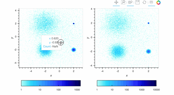
Here, the `linear` map is easy to interpret, but nearly all of the pixels are drawn in the lightest blue, because the highest-count pixel (around a count of 6000) is much larger in value than the typical pixels. The other two plots show the full structure (five concentrations of data points, including one in the background), with `log` using a standard logarithmic transformation of the count data before colormapping, and `eq_hist` using a histogram-equalization technique (see the [Datashader docs](https://datashader.org/getting_started/Pipeline.html)) to reveal structure without any assumptions about the incoming distribution (but with an irregularly spaced colormap that makes the numeric values difficult to reason about). In practice, it is generally a good idea to use `eq_hist` when exploring a large dataset initially, so that you will see any structure present, then switch to `log` or `linear` as appropriate to share the plots with a simpler-to-explain colormap. All three of these options are supported by the various backends (including Bokeh version 2.2.3 or later) and by `shade()` and `datashade()` except that `eq_hist` is not yet available for the Plotly backend.
Since datashader only sends the data currently in view to the plotting backend, the default behavior is to rescale the colormap to the range of the visible data as the zoom level changes. This behavior may not be desirable when working with images; to instead use a fixed colormap range, the `clim` parameter can be passed to the `bokeh` backend via the `opts()` method. Note that this approach works with `rasterize()` where the colormapping is done by the `bokeh` backend. With `datashade()`, the colormapping is done with the `shade()` function which takes a `clims` parameter directly instead of passing additional parameters to the backend via `opts()`. For example (removing the semicolon in a live notebook to see the output):
```python
pts1 = rasterize(hv.Points(df)).opts(**ropts).opts(tools=[], cnorm='log', axiswise=True)
pts2 = rasterize(hv.Points(df)).opts(**ropts).opts(tools=[], cnorm='log', axiswise=True)
pts1 + pts2.opts(clim=(0, 10000));
```
 By default, pixels with an integer count of zero or a floating-point value of NaN are transparent, letting the plot background show through so that the data can be used in overlays. If you want zero to map to the lowest colormap color instead to make a dense, fully filled-in image, you can use `redim.nodata` to set the `Dimension.nodata` parameter to None:
```python
hv.Layout([rasterize(hv.Points(df), vdim_prefix='').redim.nodata(Count=n)\
.opts(**ropts, cnorm="eq_hist").relabel("nodata="+str(n))
for n in [0, None]])
```
## Spreading and antialiasing
By default, Datashader treats points and lines as infinitesimal in width, such that a given point or small bit of line segment appears in at most one pixel. This approach ensures that the overall distribution of the points will be mathematically well founded -- each pixel will scale in value directly by the number of points that fall into it, or by the lines that cross it. As a consequence, Datashader's "marker size" and "line width" are effectively one pixel by default.
However, many monitors are sufficiently high resolution that a single-pixel point or line can be difficult to see---one pixel may not be visible at all on its own, and even if it is visible it is often difficult to see its color. To compensate for this, HoloViews provides access to Datashader's raster-based "spreading" (a generalization of image dilation and convolution), which makes isolated nonzero cells "spread" into adjacent ones for visibility. There are two varieties of spreading supported:
1. ``spread``: fixed spreading of a certain number of cells (pixels), which is useful if you want to be sure how much spreading is done regardless of the properties of the data.
2. ``dynspread``: spreads up to a maximum size as long as it does not exceed a specified fraction of adjacency between cells (pixels) (controlled by a `threshold` parameter).
Dynamic spreading is typically more useful for interactive plotting, because it adjusts depending on how close the datapoints are to each other on screen. As of Datashader 0.12, both types of spreading are supported for both `rasterize()` and `shade()`, but previous Datashader versions only support spreading on the RGB output of `shade()`.
As long as you have Datashader 0.12 or later, you can compare the results when you zoom the two plots below; when you zoom in far enough you should be able to see that the in the two zoomed-in plots below, then zoom out to see that the plots are the same when points are clustered together to form a distribution. (If running a live notebook; remove the semicolon so that you see the live output rather than the saved GIF.)
```python
pts = rasterize(points).opts(cnorm='eq_hist')
pts + dynspread(pts);
```
By default, pixels with an integer count of zero or a floating-point value of NaN are transparent, letting the plot background show through so that the data can be used in overlays. If you want zero to map to the lowest colormap color instead to make a dense, fully filled-in image, you can use `redim.nodata` to set the `Dimension.nodata` parameter to None:
```python
hv.Layout([rasterize(hv.Points(df), vdim_prefix='').redim.nodata(Count=n)\
.opts(**ropts, cnorm="eq_hist").relabel("nodata="+str(n))
for n in [0, None]])
```
## Spreading and antialiasing
By default, Datashader treats points and lines as infinitesimal in width, such that a given point or small bit of line segment appears in at most one pixel. This approach ensures that the overall distribution of the points will be mathematically well founded -- each pixel will scale in value directly by the number of points that fall into it, or by the lines that cross it. As a consequence, Datashader's "marker size" and "line width" are effectively one pixel by default.
However, many monitors are sufficiently high resolution that a single-pixel point or line can be difficult to see---one pixel may not be visible at all on its own, and even if it is visible it is often difficult to see its color. To compensate for this, HoloViews provides access to Datashader's raster-based "spreading" (a generalization of image dilation and convolution), which makes isolated nonzero cells "spread" into adjacent ones for visibility. There are two varieties of spreading supported:
1. ``spread``: fixed spreading of a certain number of cells (pixels), which is useful if you want to be sure how much spreading is done regardless of the properties of the data.
2. ``dynspread``: spreads up to a maximum size as long as it does not exceed a specified fraction of adjacency between cells (pixels) (controlled by a `threshold` parameter).
Dynamic spreading is typically more useful for interactive plotting, because it adjusts depending on how close the datapoints are to each other on screen. As of Datashader 0.12, both types of spreading are supported for both `rasterize()` and `shade()`, but previous Datashader versions only support spreading on the RGB output of `shade()`.
As long as you have Datashader 0.12 or later, you can compare the results when you zoom the two plots below; when you zoom in far enough you should be able to see that the in the two zoomed-in plots below, then zoom out to see that the plots are the same when points are clustered together to form a distribution. (If running a live notebook; remove the semicolon so that you see the live output rather than the saved GIF.)
```python
pts = rasterize(points).opts(cnorm='eq_hist')
pts + dynspread(pts);
```
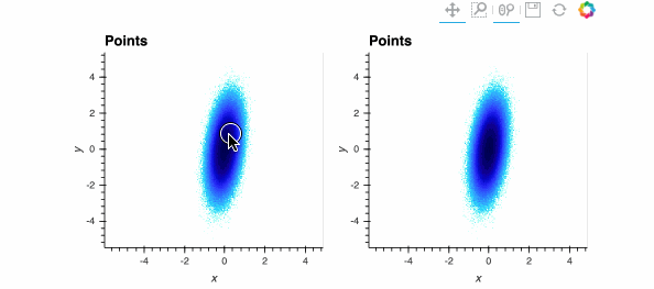 Both plots show the same data, and look identical when zoomed out, but when zoomed in enough you should be able to see the individual data points on the right while the ones on the left are barely visible. The dynspread parameters typically need some hand tuning, as the only purpose of such spreading is to make things visible on a particular monitor for a particular observer; the underlying mathematical operations in Datashader do not normally need parameters to be adjusted.
Dynspread is not usable with connected plots like trajectories or curves, because the spreading amount is measured by the fraction of cells that have neighbors closer than the given spread distance, which is always 100% when datapoints are connected together. For connected plots you can instead use `spread` with a fixed value to expand patterns by `px` in every direction after they are drawn, or (for Datashader 0.14 or later) pass an explicit width like `line_width=1` to the rasterizer (at some cost in performance) to draw fully antialiased lines with the specified width:
```python
rasterize(paths).relabel("Rasterized") + \
spread(rasterize(paths), px=1).relabel("Spread 1") + \
rasterize(paths, line_width=2).relabel("Antialiased line_width 2")
```
# Multidimensional plots
The above plots show two dimensions of data plotted along *x* and *y*, but Datashader operations can be used with additional dimensions as well. For instance, an extra dimension (here called `k`), can be treated as a category label and used to colorize the points or lines, aggregating the data points separately depending on which category value they have. Compared to a standard overlaid scatterplot that would suffer from overplotting, here the result will be merged mathematically by Datashader, completely avoiding any overplotting issues except any local issues that may arise from spreading when zoomed in:
```python
np.random.seed(3)
kdims=['d1','d2']
num_ks=8
def rand_gauss2d(value=0, n=100000):
"""Return a randomly shaped 2D Gaussian distribution with an associated numeric value"""
g = 100*np.random.multivariate_normal(np.random.randn(2), random_cov(), (n,))
return np.hstack((g,value*np.ones((g.shape[0],1))))
```
```python
gaussians = {str(i): hv.Points(rand_gauss2d(i), kdims, "i") for i in range(num_ks)}
c = dynspread(datashade(hv.NdOverlay(gaussians, kdims='k'), aggregator=ds.by('k', ds.count())))
m = dynspread(datashade(hv.NdOverlay(gaussians, kdims='k'), aggregator=ds.by('k', ds.mean("i"))))
c.opts(width=400) + m.opts(width=400)
```
Above you can see that (as of Datashader 0.11) categorical aggregates can take any reduction function, either `count`ing the datapoints (left) or reporting some other statistic (e.g. the mean value of a column, right). This type of categorical mixing is currently only supported by `shade()` and `datashade()`, not `rasterize()` alone, because it depends on Datashader's custom color mixing code.
Categorical aggregates are one way to allow separate lines or other shapes to be visually distinctive from one another while avoiding obscuring data due to overplotting:
```python
lines = {str(i): hv.Curve(time_series(N=10000, S0=200+np.random.rand())) for i in range(num_ks)}
lineoverlay = hv.NdOverlay(lines, kdims='k')
datashade(lineoverlay, pixel_ratio=2, line_width=4, aggregator=ds.by('k', ds.count())).opts(width=800)
```
As you can see, overlapping colors yield color mixtures that indicate that the given pixels contain data from multiple curves, which helps users realize where they need to zoom in to see further detail.
Note that Bokeh only ever sees an image come out of `datashade`, not any of the actual data. As a result, providing legends and keys has to be done separately, though we are hoping to make this process more seamless. For now, you can show a legend by adding a suitable collection of "fake" labeled points (size zero and thus invisible):
```python
# definition copied here to ensure independent pan/zoom state for each dynamic plot
gaussspread2 = dynspread(datashade(hv.NdOverlay(gaussians, kdims=['k']), aggregator=ds.by('k', ds.count())))
from datashader.colors import Sets1to3 # default datashade() and shade() color cycle
color_key = list(enumerate(Sets1to3[0:num_ks]))
color_points = hv.NdOverlay({k: hv.Points([(0,0)], label=str(k)).opts(color=v, size=0) for k, v in color_key})
(color_points * gaussspread2).opts(width=600)
```
Here the dummy points are at (0,0) for this dataset, but would need to be at another suitable value for data that is in a different range.
## Working with time series
HoloViews also makes it possible to datashade large timeseries using the ``datashade`` and ``rasterize`` operations. For smoother lines, datashader implements anti-aliasing if a `line_width` > 0 is set:
```python
dates = pd.date_range(start="2014-01-01", end="2016-01-01", freq='1D') # or '1min'
curve = hv.Curve((dates, time_series(N=len(dates), sigma = 1)))
rasterize(curve, width=800, line_width=3, pixel_ratio=2).opts(width=800, cmap=['lightblue','blue'])
```
Here we're also doubling the resolution in x and y using `pixel_ratio=2`, allowing for more precise rendering of the line shape; higher pixel ratios work well for lines and other shapes, though they can make individual points more difficult to see in points plots.
HoloViews also supplies some operations that are useful in combination with Datashader timeseries. For instance, you can compute a rolling mean of the results and then show a subset of outlier points, which will then support hover, selection, and other interactive Bokeh features:
```python
from holoviews.operation.timeseries import rolling, rolling_outlier_std
smoothed = rolling(curve, rolling_window=50)
outliers = rolling_outlier_std(curve, rolling_window=50, sigma=2)
ds_curve = rasterize(curve, line_width=2.5, pixel_ratio=2).opts(cmap=["lightblue","blue"])
curvespread = rasterize(smoothed, line_width=6, pixel_ratio=2).opts(cmap=["pink","red"], width=800)
(ds_curve * curvespread * outliers).opts(
opts.Scatter(line_color="black", fill_color="red", size=10, tools=['hover', 'box_select'], width=800))
```
Another option when working with time series is to downsample the data before plotting it. This can be done with `downsample1D`. Algorithms supported are `lttb` (Largest Triangle Three Buckets) and `nth` element. The two algorithm is overlaid on top of the original curve in the example below.
```python
from holoviews.operation.downsample import downsample1d
lttb = downsample1d(curve)
nth = downsample1d(curve, algorithm="nth")
lttb_com = (curve * lttb).opts(width=800, title="lttb comparison")
nth_com = (curve * nth).opts(width=800, title="nth comparison")
(lttb_com + nth_com).cols(1)
```
The result of all these operations can be laid out, overlaid, selected, and sampled just like any other HoloViews element, letting you work naturally with even very large datasets.
Note that the above plot will look blocky in a static export (such as on anaconda.org), because the exported version is generated without taking the size of the actual plot (using default height and width for Datashader) into account, whereas the live notebook automatically regenerates the plot to match the visible area on the page.
# Element types supported for Datashading
Fundamentally, what Datashader does is to rasterize data, i.e., render a representation of it into a regularly gridded rectangular portion of a two-dimensional plane. Datashader natively supports six basic types of rasterization:
- **points**: zero-dimensional objects aggregated by position alone, each point covering zero area in the plane and thus falling into exactly one grid cell of the resulting array (if the point is within the bounds being aggregated).
- **line**: polyline/multiline objects (connected series of line segments), with each segment having a fixed length but either zero width (not antialiased) or a specified width, and crossing each grid cell at most once.
- **area**: a region to fill either between the supplied y-values and the origin or between two supplied lines.
- **trimesh**: irregularly spaced triangular grid, with each triangle covering a portion of the 2D plane and thus potentially crossing multiple grid cells (thus requiring interpolation/upsampling). Depending on the zoom level, a single pixel can also include multiple triangles, which then becomes similar to the `points` case (requiring aggregation/downsampling of all triangles covered by the pixel).
- **raster**: an axis-aligned regularly gridded two-dimensional subregion of the plane, with each grid cell in the source data covering more than one grid cell in the output grid (requiring interpolation/upsampling), or with each grid cell in the output grid including contributions from more than one grid cell in the input grid (requiring aggregation/downsampling).
- **quadmesh**: a recti-linear or curvi-linear mesh (like a raster, but allowing nonuniform spacing and coordinate mapping) where each quad can cover one or more cells in the output (requiring upsampling, currently only as nearest neighbor), or with each output grid cell including contributions from more than one input grid cell (requiring aggregation/downsampling).
- **polygons**: arbitrary filled shapes in 2D space (bounded by a piecewise linear set of segments), optionally punctuated by similarly bounded internal holes.
Datashader focuses on implementing those four cases very efficiently, and HoloViews in turn can use them to render a very large range of specific types of data:
### Supported Elements
- **points**: [`hv.Nodes`](../reference/elements/bokeh/Graph.ipynb), [`hv.Points`](../reference/elements/bokeh/Points.ipynb), [`hv.Scatter`](../reference/elements/bokeh/Scatter.ipynb)
- **line**: [`hv.Contours`](../reference/elements/bokeh/Contours.ipynb), [`hv.Curve`](../reference/elements/bokeh/Curve.ipynb), [`hv.Path`](../reference/elements/bokeh/Path.ipynb), [`hv.Graph`](../reference/elements/bokeh/Graph.ipynb), [`hv.EdgePaths`](../reference/elements/bokeh/Graph.ipynb), [`hv.Spikes`](../reference/elements/bokeh/Spikes.ipynb), [`hv.Segments`](../reference/elements/bokeh/Segments.ipynb)
- **area**: [`hv.Area`](../reference/elements/bokeh/Area.ipynb), [`hv.Rectangles`](../reference/elements/bokeh/Rectangles.ipynb), [`hv.Spread`](../reference/elements/bokeh/Spread.ipynb)
- **raster**: [`hv.Image`](../reference/elements/bokeh/Image.ipynb), [`hv.HSV`](../reference/elements/bokeh/HSV.ipynb), [`hv.RGB`](../reference/elements/bokeh/RGB.ipynb)
- **trimesh**: [`hv.TriMesh`](../reference/elements/bokeh/TriMesh.ipynb)
- **quadmesh**: [`hv.QuadMesh`](../reference/elements/bokeh/QuadMesh.ipynb)
- **polygons**: [`hv.Polygons`](../reference/elements/bokeh/Polygons.ipynb)
Other HoloViews elements *could* be supported, but do not currently have a useful datashaded representation:
### Elements not yet supported
- **line**: [`hv.Spline`](../reference/elements/bokeh/Spline.ipynb), [`hv.VectorField`](../reference/elements/bokeh/VectorField.ipynb)
- **raster**: [`hv.HeatMap`](../reference/elements/bokeh/HeatMap.ipynb), [`hv.Raster`](../reference/elements/bokeh/Raster.ipynb)
There are also other Elements that are not expected to be useful with datashader because they are isolated annotations, are already summaries or aggregations of other data, have graphical representations that are only meaningful at a certain size, or are text based:
### Not useful to support
- datashadable annotations: [`hv.Arrow`](../reference/elements/bokeh/Arrow.ipynb), [`hv.Bounds`](../reference/elements/bokeh/Bounds.ipynb), [`hv.Box`](../reference/elements/bokeh/Box.ipynb), [`hv.Ellipse`](../reference/elements/bokeh/Ellipse.ipynb) (actually do work with datashade currently, but not officially supported because they are not vectorized and thus unlikely to have enough items to be worth datashading)
- other annotations: [`hv.Labels`](../reference/elements/bokeh/Labels.ipynb), [`hv.HLine`](../reference/elements/bokeh/HLine.ipynb), [`hv.VLine`](../reference/elements/bokeh/VLine.ipynb), [`hv.Text`](../reference/elements/bokeh/Text.ipynb)
- kdes: [`hv.Distribution`](../reference/elements/bokeh/Distribution.ipynb), [`hv.Bivariate`](../reference/elements/bokeh/Bivariate.ipynb) (already aggregated)
- categorical/symbolic: [`hv.BoxWhisker`](../reference/elements/bokeh/BoxWhisker.ipynb), [`hv.Bars`](../reference/elements/bokeh/Bars.ipynb), [`hv.ErrorBars`](../reference/elements/bokeh/ErrorBars.ipynb)
- tables: [`hv.Table`](../reference/elements/bokeh/Table.ipynb), [`hv.ItemTable`](../reference/elements/bokeh/ItemTable.ipynb)
Let's make some examples of each supported Element type. First, some dummy data:
```python
from bokeh.sampledata.unemployment import data as unemployment
from bokeh.sampledata.us_counties import data as counties
np.random.seed(12)
N=50
pts = [(10*i/N, np.sin(10*i/N)) for i in range(N)]
x = y = np.linspace(0, 5, int(np.sqrt(N)))
xs,ys = np.meshgrid(x,y)
z = np.sin(xs)*np.cos(ys)
r = 0.5*np.sin(0.1*xs**2+0.05*ys**2)+0.5
g = 0.5*np.sin(0.02*xs**2+0.2*ys**2)+0.5
b = 0.5*np.sin(0.02*xs**2+0.02*ys**2)+0.5
n=20
coords = np.linspace(-1.5,1.5,n)
X,Y = np.meshgrid(coords, coords);
Qx = np.cos(Y) - np.cos(X)
Qy = np.sin(Y) + np.sin(X)
Z = np.sqrt(X**2 + Y**2)
rect_colors = {True: 'red', False: 'green'}
s = np.random.randn(100).cumsum()
e = s + np.random.randn(100)
```
Next, some options:
```python
hv.output(backend='matplotlib')
opts.defaults(opts.Layout(vspace=0.1, hspace=0.1, sublabel_format='', fig_size=48))
eopts = dict(aspect=1, axiswise=True, xaxis='bare', yaxis='bare', xticks=False, yticks=False)
opts2 = dict(filled=True, edge_color='z')
rect_opts = opts.Rectangles(lw=0, color=hv.dim('sign').categorize(rect_colors))
ds_point_opts = dict(aggregator='any')
ds_line_opts = dict(aggregator='any', line_width=1)
ResampleOperation2D.width=115
ResampleOperation2D.height=115
ds_opts = {
hv.Path: ds_line_opts,
hv.Graph: ds_line_opts,
hv.Contours: ds_line_opts,
hv.EdgePaths: ds_line_opts,
hv.Curve: ds_line_opts,
hv.Scatter: ds_point_opts,
hv.Points: ds_point_opts,
hv.Segments: ds_point_opts,
hv.Rectangles: dict(aggregator=ds.count_cat('sign'), color_key=rect_colors)
}
```
Now, some Elements that support datashading, in categories depending on whether they work best with `spread(rasterize())`, with plain `rasterize()`, or require `datashade()`:
```python
tri = hv.TriMesh.from_vertices(hv.Points(np.random.randn(N,3), vdims='z')).opts(**opts2)
rasterizable = [hv.Curve(pts)]
rasterizable += [hv.operation.contours(hv.Image((x,y,z)), levels=10)]
rasterizable += [hv.Area(np.random.randn(10000).cumsum())]
rasterizable += [hv.Spread((np.arange(10000), np.random.randn(10000).cumsum(), np.random.randn(10000)*10))]
rasterizable += [hv.Spikes(np.random.randn(1000))]
rasterizable += [hv.Graph(((np.zeros(N//2), np.arange(N//2)),))]
rasterizable += [hv.QuadMesh((Qx,Qy,Z))]
rasterizable += [hv.Image((x,y,z))]
rasterizable += [hv.RGB(np.dstack([r,g,b])), hv.HSV(np.dstack([g,b,r]))]
rasterizable += [tri, tri.edgepaths]
rasterizable += [hv.Path(counties[(1, 1)], ['lons', 'lats'])]
polys = hv.Polygons([dict(county, unemployment=unemployment[k])
for k, county in counties.items()
if county['state'] == 'tx'],
['lons', 'lats'], ['unemployment']).opts(color='unemployment')
try:
import spatialpandas # Needed for datashader polygon support
rasterizable += [polys]
except: pass
spreadable = [e(pts) for e in [hv.Scatter]]
spreadable += [hv.Points(counties[(1, 1)], ['lons', 'lats'])]
spreadable += [hv.Segments((np.arange(100), s, np.arange(100), e))]
shadeable = [hv.Rectangles((np.arange(100)-0.4, s, np.arange(100)+0.4, e, s>e), vdims='sign').opts(rect_opts)]
```
We can now view these with Datashader via `spread(rasterize())`, `rasterize()`, or `datashade()`:
```python
def nop(x,**k): return x
def spread2(e, **k): return spread(rasterize(e, **k), px=2).opts(cnorm='eq_hist', padding=0.1)
def plot(e, operation=nop):
return operation(e.relabel(e.__class__.name), **ds_opts.get(e.__class__, {})).opts(**eopts)
hv.Layout(
[plot(e, rasterize) for e in rasterizable] + \
[plot(e, spread2) for e in spreadable] + \
[plot(e, datashade) for e in shadeable]).cols(6)
```
For comparison, you can see the corresponding non-datashaded plots (as long as you leave N lower than 10000 unless you have a long time to wait!):
```python
hv.Layout([plot(e) for e in rasterizable + spreadable + shadeable]).cols(6)
```
The previous two sets of examples use Matplotlib, but if they were switched to Bokeh and you had a live server, they would support dynamic re-rendering on zoom and pan so that you could explore the full range of data available (e.g. even very large raster images, networks, paths, point clouds, or meshes).
```python
hv.output(backend='bokeh') # restore bokeh backend in case cells will run out of order
```
# Container types supported for datashading
In the above examples `datashade()` or `rasterize` was called directly on each Element, but these operations can also be called on Containers, in which case each Element in the Container will be datashaded separately (for all Container types other than a Layout):
```python
curves = {'+':hv.Curve(pts), '-':hv.Curve([(x, -1.0*y) for x, y in pts])}
rasterize(hv.HoloMap(curves,'sign'), line_width=3)
```
```python
rasterize(hv.NdLayout(curves,'sign'), line_width=3)
```
```python
containers = [hv.Overlay(list(curves.values())), hv.NdOverlay(curves), hv.GridSpace(hv.NdOverlay(curves))]
hv.Layout([rasterize(e.relabel(e.__class__.name), line_width=3) for e in containers]).cols(3)
```
# Optimizing performance
Datashader and HoloViews have different design principles that are worth keeping in mind when using them in combination, if you want to ensure good overall performance. By design, Datashader supports only a small number of operations and datatypes, focusing only on what can be implemented very efficiently. HoloViews instead focuses on supporting the typical workflows of Python users, recognizing that the most computationally efficient choice is only going to be faster overall if it also minimizes the time users have to spend getting things working.
HoloViews thus helps you get something working quickly, but once it is working and you realize that you need to do this often or that it comes up against the limits of your computing hardware, you can consider whether you can get much better performance by considering the following issues and suggestions.
### Use a Datashader-supported data structure
HoloViews helpfully tries to convert whatever data you have provided into what Datashader supports, which is good for optimizing your time to an initial solution, but will not always be the fastest approach computationally. If you ensure that you store your data in a format that Datashader understands already, HoloViews can simply pass it down to Datashader without copying or transforming it:
1. For point, line, and trimesh data, Datashader supports Dask and Pandas dataframes, and so those two data sources will be fastest. Of those two, Dask Dataframes will usually be somewhat faster and also able to make use of distributed computational resources and out-of-core processing.
2. For rasters and quadmeshes, Datashader supports xarray objects natively, and so if your data is provided as an xarray already, plotting will be faster.
3. For polygons Datashader supports [spatialpandas](https://github.com/holoviz/spatialpandas) DataFrames.
See the [Datashader docs](http://datashader.org) for examples of dealing with even quite large datasets (in the billions of points) on commodity hardware, including many HoloViews-based examples.
### Cache initial processing with `precompute=True`
In the typical case of having datasets much larger than the plot resolution, HoloViews Datashader-based operations that work on the full dataset (`rasterize`, `aggregate`,`regrid`) are computationally expensive; the others are not (`shade`, `spread`, `dynspread`, etc.)
The expensive operations are all of type `ResamplingOperation`, which has a parameter `precompute` (see `hv.help(hv.operation.datashader.rasterize)`, etc.) Precompute can be used to get faster performance in interactive usage by caching the last set of data used in plotting (*after* any transformations needed) and reusing it when it is requested again. This is particularly useful when your data is not in one of the supported data formats already and needs to be converted. `precompute` is False by default, because it requires using memory to store the cached data, but if you have enough memory, you can enable it so that repeated interactions (such as zooming and panning) will be much faster than the first one. In practice, most Datashader-plots don't need to do extensive precomputing, but enabling it for TriMesh and Polygon plots can greatly speed up interactive usage.
### Use GPU support
Many elements now also support aggregation directly on a GPU-based datastructure such as a [cuDF DataFrame](https://github.com/rapidsai/cudf) or an Xarray DataArray backed by a [cupy](https://github.com/cupy/cupy) array. These data structures can be passed directly to the appropriate HoloViews elements just as you would use a Pandas or other Xarray object. For instance, a cuDF can be used on elements like `hv.Points` and `hv.Curve`, while a cupy-backed DataArray raster or quadmesh can be passed to `hv.QuadMesh` elements. When used with Datashader, the GPU implementation can result in 10-100x speedups, as well as avoiding having to transfer the data out of the GPU for plotting (sending only the final rendered plot out of the GPU's memory). To see which HoloViews elements are supported, see the [datashader performance guide](https://datashader.org/user_guide/Performance.html). As of the Datashader 0.11 release, all point, line, area, and quadmesh aggregations are supported when using a GPU backed datastructure, including raster objects like `hv.Image` if first converted to `hv.Quadmesh`.
### Project data only once
If you are working with geographic data using [GeoViews](http://geoviews.org) that needs to be projected before display and/or before datashading, GeoViews will have to do this every time you update a plot, which can drown out the performance improvement you get by using Datashader. GeoViews allows you to project the entire dataset at once using `gv.operation.project`, and once you do this you should be able to use Datashader at full speed.
If you follow these suggestions, the combination of HoloViews and Datashader will allow you to work uniformly with data covering a huge range of sizes. Per session or per plot, you can trade off the ability to export user-manipulable plots against file size and browser compatibility, and allowing you to render even the largest dataset faithfully. HoloViews makes the full power of Datashader available in just a few lines of code, giving you a natural way to work with your data regardless of its size.
Both plots show the same data, and look identical when zoomed out, but when zoomed in enough you should be able to see the individual data points on the right while the ones on the left are barely visible. The dynspread parameters typically need some hand tuning, as the only purpose of such spreading is to make things visible on a particular monitor for a particular observer; the underlying mathematical operations in Datashader do not normally need parameters to be adjusted.
Dynspread is not usable with connected plots like trajectories or curves, because the spreading amount is measured by the fraction of cells that have neighbors closer than the given spread distance, which is always 100% when datapoints are connected together. For connected plots you can instead use `spread` with a fixed value to expand patterns by `px` in every direction after they are drawn, or (for Datashader 0.14 or later) pass an explicit width like `line_width=1` to the rasterizer (at some cost in performance) to draw fully antialiased lines with the specified width:
```python
rasterize(paths).relabel("Rasterized") + \
spread(rasterize(paths), px=1).relabel("Spread 1") + \
rasterize(paths, line_width=2).relabel("Antialiased line_width 2")
```
# Multidimensional plots
The above plots show two dimensions of data plotted along *x* and *y*, but Datashader operations can be used with additional dimensions as well. For instance, an extra dimension (here called `k`), can be treated as a category label and used to colorize the points or lines, aggregating the data points separately depending on which category value they have. Compared to a standard overlaid scatterplot that would suffer from overplotting, here the result will be merged mathematically by Datashader, completely avoiding any overplotting issues except any local issues that may arise from spreading when zoomed in:
```python
np.random.seed(3)
kdims=['d1','d2']
num_ks=8
def rand_gauss2d(value=0, n=100000):
"""Return a randomly shaped 2D Gaussian distribution with an associated numeric value"""
g = 100*np.random.multivariate_normal(np.random.randn(2), random_cov(), (n,))
return np.hstack((g,value*np.ones((g.shape[0],1))))
```
```python
gaussians = {str(i): hv.Points(rand_gauss2d(i), kdims, "i") for i in range(num_ks)}
c = dynspread(datashade(hv.NdOverlay(gaussians, kdims='k'), aggregator=ds.by('k', ds.count())))
m = dynspread(datashade(hv.NdOverlay(gaussians, kdims='k'), aggregator=ds.by('k', ds.mean("i"))))
c.opts(width=400) + m.opts(width=400)
```
Above you can see that (as of Datashader 0.11) categorical aggregates can take any reduction function, either `count`ing the datapoints (left) or reporting some other statistic (e.g. the mean value of a column, right). This type of categorical mixing is currently only supported by `shade()` and `datashade()`, not `rasterize()` alone, because it depends on Datashader's custom color mixing code.
Categorical aggregates are one way to allow separate lines or other shapes to be visually distinctive from one another while avoiding obscuring data due to overplotting:
```python
lines = {str(i): hv.Curve(time_series(N=10000, S0=200+np.random.rand())) for i in range(num_ks)}
lineoverlay = hv.NdOverlay(lines, kdims='k')
datashade(lineoverlay, pixel_ratio=2, line_width=4, aggregator=ds.by('k', ds.count())).opts(width=800)
```
As you can see, overlapping colors yield color mixtures that indicate that the given pixels contain data from multiple curves, which helps users realize where they need to zoom in to see further detail.
Note that Bokeh only ever sees an image come out of `datashade`, not any of the actual data. As a result, providing legends and keys has to be done separately, though we are hoping to make this process more seamless. For now, you can show a legend by adding a suitable collection of "fake" labeled points (size zero and thus invisible):
```python
# definition copied here to ensure independent pan/zoom state for each dynamic plot
gaussspread2 = dynspread(datashade(hv.NdOverlay(gaussians, kdims=['k']), aggregator=ds.by('k', ds.count())))
from datashader.colors import Sets1to3 # default datashade() and shade() color cycle
color_key = list(enumerate(Sets1to3[0:num_ks]))
color_points = hv.NdOverlay({k: hv.Points([(0,0)], label=str(k)).opts(color=v, size=0) for k, v in color_key})
(color_points * gaussspread2).opts(width=600)
```
Here the dummy points are at (0,0) for this dataset, but would need to be at another suitable value for data that is in a different range.
## Working with time series
HoloViews also makes it possible to datashade large timeseries using the ``datashade`` and ``rasterize`` operations. For smoother lines, datashader implements anti-aliasing if a `line_width` > 0 is set:
```python
dates = pd.date_range(start="2014-01-01", end="2016-01-01", freq='1D') # or '1min'
curve = hv.Curve((dates, time_series(N=len(dates), sigma = 1)))
rasterize(curve, width=800, line_width=3, pixel_ratio=2).opts(width=800, cmap=['lightblue','blue'])
```
Here we're also doubling the resolution in x and y using `pixel_ratio=2`, allowing for more precise rendering of the line shape; higher pixel ratios work well for lines and other shapes, though they can make individual points more difficult to see in points plots.
HoloViews also supplies some operations that are useful in combination with Datashader timeseries. For instance, you can compute a rolling mean of the results and then show a subset of outlier points, which will then support hover, selection, and other interactive Bokeh features:
```python
from holoviews.operation.timeseries import rolling, rolling_outlier_std
smoothed = rolling(curve, rolling_window=50)
outliers = rolling_outlier_std(curve, rolling_window=50, sigma=2)
ds_curve = rasterize(curve, line_width=2.5, pixel_ratio=2).opts(cmap=["lightblue","blue"])
curvespread = rasterize(smoothed, line_width=6, pixel_ratio=2).opts(cmap=["pink","red"], width=800)
(ds_curve * curvespread * outliers).opts(
opts.Scatter(line_color="black", fill_color="red", size=10, tools=['hover', 'box_select'], width=800))
```
Another option when working with time series is to downsample the data before plotting it. This can be done with `downsample1D`. Algorithms supported are `lttb` (Largest Triangle Three Buckets) and `nth` element. The two algorithm is overlaid on top of the original curve in the example below.
```python
from holoviews.operation.downsample import downsample1d
lttb = downsample1d(curve)
nth = downsample1d(curve, algorithm="nth")
lttb_com = (curve * lttb).opts(width=800, title="lttb comparison")
nth_com = (curve * nth).opts(width=800, title="nth comparison")
(lttb_com + nth_com).cols(1)
```
The result of all these operations can be laid out, overlaid, selected, and sampled just like any other HoloViews element, letting you work naturally with even very large datasets.
Note that the above plot will look blocky in a static export (such as on anaconda.org), because the exported version is generated without taking the size of the actual plot (using default height and width for Datashader) into account, whereas the live notebook automatically regenerates the plot to match the visible area on the page.
# Element types supported for Datashading
Fundamentally, what Datashader does is to rasterize data, i.e., render a representation of it into a regularly gridded rectangular portion of a two-dimensional plane. Datashader natively supports six basic types of rasterization:
- **points**: zero-dimensional objects aggregated by position alone, each point covering zero area in the plane and thus falling into exactly one grid cell of the resulting array (if the point is within the bounds being aggregated).
- **line**: polyline/multiline objects (connected series of line segments), with each segment having a fixed length but either zero width (not antialiased) or a specified width, and crossing each grid cell at most once.
- **area**: a region to fill either between the supplied y-values and the origin or between two supplied lines.
- **trimesh**: irregularly spaced triangular grid, with each triangle covering a portion of the 2D plane and thus potentially crossing multiple grid cells (thus requiring interpolation/upsampling). Depending on the zoom level, a single pixel can also include multiple triangles, which then becomes similar to the `points` case (requiring aggregation/downsampling of all triangles covered by the pixel).
- **raster**: an axis-aligned regularly gridded two-dimensional subregion of the plane, with each grid cell in the source data covering more than one grid cell in the output grid (requiring interpolation/upsampling), or with each grid cell in the output grid including contributions from more than one grid cell in the input grid (requiring aggregation/downsampling).
- **quadmesh**: a recti-linear or curvi-linear mesh (like a raster, but allowing nonuniform spacing and coordinate mapping) where each quad can cover one or more cells in the output (requiring upsampling, currently only as nearest neighbor), or with each output grid cell including contributions from more than one input grid cell (requiring aggregation/downsampling).
- **polygons**: arbitrary filled shapes in 2D space (bounded by a piecewise linear set of segments), optionally punctuated by similarly bounded internal holes.
Datashader focuses on implementing those four cases very efficiently, and HoloViews in turn can use them to render a very large range of specific types of data:
### Supported Elements
- **points**: [`hv.Nodes`](../reference/elements/bokeh/Graph.ipynb), [`hv.Points`](../reference/elements/bokeh/Points.ipynb), [`hv.Scatter`](../reference/elements/bokeh/Scatter.ipynb)
- **line**: [`hv.Contours`](../reference/elements/bokeh/Contours.ipynb), [`hv.Curve`](../reference/elements/bokeh/Curve.ipynb), [`hv.Path`](../reference/elements/bokeh/Path.ipynb), [`hv.Graph`](../reference/elements/bokeh/Graph.ipynb), [`hv.EdgePaths`](../reference/elements/bokeh/Graph.ipynb), [`hv.Spikes`](../reference/elements/bokeh/Spikes.ipynb), [`hv.Segments`](../reference/elements/bokeh/Segments.ipynb)
- **area**: [`hv.Area`](../reference/elements/bokeh/Area.ipynb), [`hv.Rectangles`](../reference/elements/bokeh/Rectangles.ipynb), [`hv.Spread`](../reference/elements/bokeh/Spread.ipynb)
- **raster**: [`hv.Image`](../reference/elements/bokeh/Image.ipynb), [`hv.HSV`](../reference/elements/bokeh/HSV.ipynb), [`hv.RGB`](../reference/elements/bokeh/RGB.ipynb)
- **trimesh**: [`hv.TriMesh`](../reference/elements/bokeh/TriMesh.ipynb)
- **quadmesh**: [`hv.QuadMesh`](../reference/elements/bokeh/QuadMesh.ipynb)
- **polygons**: [`hv.Polygons`](../reference/elements/bokeh/Polygons.ipynb)
Other HoloViews elements *could* be supported, but do not currently have a useful datashaded representation:
### Elements not yet supported
- **line**: [`hv.Spline`](../reference/elements/bokeh/Spline.ipynb), [`hv.VectorField`](../reference/elements/bokeh/VectorField.ipynb)
- **raster**: [`hv.HeatMap`](../reference/elements/bokeh/HeatMap.ipynb), [`hv.Raster`](../reference/elements/bokeh/Raster.ipynb)
There are also other Elements that are not expected to be useful with datashader because they are isolated annotations, are already summaries or aggregations of other data, have graphical representations that are only meaningful at a certain size, or are text based:
### Not useful to support
- datashadable annotations: [`hv.Arrow`](../reference/elements/bokeh/Arrow.ipynb), [`hv.Bounds`](../reference/elements/bokeh/Bounds.ipynb), [`hv.Box`](../reference/elements/bokeh/Box.ipynb), [`hv.Ellipse`](../reference/elements/bokeh/Ellipse.ipynb) (actually do work with datashade currently, but not officially supported because they are not vectorized and thus unlikely to have enough items to be worth datashading)
- other annotations: [`hv.Labels`](../reference/elements/bokeh/Labels.ipynb), [`hv.HLine`](../reference/elements/bokeh/HLine.ipynb), [`hv.VLine`](../reference/elements/bokeh/VLine.ipynb), [`hv.Text`](../reference/elements/bokeh/Text.ipynb)
- kdes: [`hv.Distribution`](../reference/elements/bokeh/Distribution.ipynb), [`hv.Bivariate`](../reference/elements/bokeh/Bivariate.ipynb) (already aggregated)
- categorical/symbolic: [`hv.BoxWhisker`](../reference/elements/bokeh/BoxWhisker.ipynb), [`hv.Bars`](../reference/elements/bokeh/Bars.ipynb), [`hv.ErrorBars`](../reference/elements/bokeh/ErrorBars.ipynb)
- tables: [`hv.Table`](../reference/elements/bokeh/Table.ipynb), [`hv.ItemTable`](../reference/elements/bokeh/ItemTable.ipynb)
Let's make some examples of each supported Element type. First, some dummy data:
```python
from bokeh.sampledata.unemployment import data as unemployment
from bokeh.sampledata.us_counties import data as counties
np.random.seed(12)
N=50
pts = [(10*i/N, np.sin(10*i/N)) for i in range(N)]
x = y = np.linspace(0, 5, int(np.sqrt(N)))
xs,ys = np.meshgrid(x,y)
z = np.sin(xs)*np.cos(ys)
r = 0.5*np.sin(0.1*xs**2+0.05*ys**2)+0.5
g = 0.5*np.sin(0.02*xs**2+0.2*ys**2)+0.5
b = 0.5*np.sin(0.02*xs**2+0.02*ys**2)+0.5
n=20
coords = np.linspace(-1.5,1.5,n)
X,Y = np.meshgrid(coords, coords);
Qx = np.cos(Y) - np.cos(X)
Qy = np.sin(Y) + np.sin(X)
Z = np.sqrt(X**2 + Y**2)
rect_colors = {True: 'red', False: 'green'}
s = np.random.randn(100).cumsum()
e = s + np.random.randn(100)
```
Next, some options:
```python
hv.output(backend='matplotlib')
opts.defaults(opts.Layout(vspace=0.1, hspace=0.1, sublabel_format='', fig_size=48))
eopts = dict(aspect=1, axiswise=True, xaxis='bare', yaxis='bare', xticks=False, yticks=False)
opts2 = dict(filled=True, edge_color='z')
rect_opts = opts.Rectangles(lw=0, color=hv.dim('sign').categorize(rect_colors))
ds_point_opts = dict(aggregator='any')
ds_line_opts = dict(aggregator='any', line_width=1)
ResampleOperation2D.width=115
ResampleOperation2D.height=115
ds_opts = {
hv.Path: ds_line_opts,
hv.Graph: ds_line_opts,
hv.Contours: ds_line_opts,
hv.EdgePaths: ds_line_opts,
hv.Curve: ds_line_opts,
hv.Scatter: ds_point_opts,
hv.Points: ds_point_opts,
hv.Segments: ds_point_opts,
hv.Rectangles: dict(aggregator=ds.count_cat('sign'), color_key=rect_colors)
}
```
Now, some Elements that support datashading, in categories depending on whether they work best with `spread(rasterize())`, with plain `rasterize()`, or require `datashade()`:
```python
tri = hv.TriMesh.from_vertices(hv.Points(np.random.randn(N,3), vdims='z')).opts(**opts2)
rasterizable = [hv.Curve(pts)]
rasterizable += [hv.operation.contours(hv.Image((x,y,z)), levels=10)]
rasterizable += [hv.Area(np.random.randn(10000).cumsum())]
rasterizable += [hv.Spread((np.arange(10000), np.random.randn(10000).cumsum(), np.random.randn(10000)*10))]
rasterizable += [hv.Spikes(np.random.randn(1000))]
rasterizable += [hv.Graph(((np.zeros(N//2), np.arange(N//2)),))]
rasterizable += [hv.QuadMesh((Qx,Qy,Z))]
rasterizable += [hv.Image((x,y,z))]
rasterizable += [hv.RGB(np.dstack([r,g,b])), hv.HSV(np.dstack([g,b,r]))]
rasterizable += [tri, tri.edgepaths]
rasterizable += [hv.Path(counties[(1, 1)], ['lons', 'lats'])]
polys = hv.Polygons([dict(county, unemployment=unemployment[k])
for k, county in counties.items()
if county['state'] == 'tx'],
['lons', 'lats'], ['unemployment']).opts(color='unemployment')
try:
import spatialpandas # Needed for datashader polygon support
rasterizable += [polys]
except: pass
spreadable = [e(pts) for e in [hv.Scatter]]
spreadable += [hv.Points(counties[(1, 1)], ['lons', 'lats'])]
spreadable += [hv.Segments((np.arange(100), s, np.arange(100), e))]
shadeable = [hv.Rectangles((np.arange(100)-0.4, s, np.arange(100)+0.4, e, s>e), vdims='sign').opts(rect_opts)]
```
We can now view these with Datashader via `spread(rasterize())`, `rasterize()`, or `datashade()`:
```python
def nop(x,**k): return x
def spread2(e, **k): return spread(rasterize(e, **k), px=2).opts(cnorm='eq_hist', padding=0.1)
def plot(e, operation=nop):
return operation(e.relabel(e.__class__.name), **ds_opts.get(e.__class__, {})).opts(**eopts)
hv.Layout(
[plot(e, rasterize) for e in rasterizable] + \
[plot(e, spread2) for e in spreadable] + \
[plot(e, datashade) for e in shadeable]).cols(6)
```
For comparison, you can see the corresponding non-datashaded plots (as long as you leave N lower than 10000 unless you have a long time to wait!):
```python
hv.Layout([plot(e) for e in rasterizable + spreadable + shadeable]).cols(6)
```
The previous two sets of examples use Matplotlib, but if they were switched to Bokeh and you had a live server, they would support dynamic re-rendering on zoom and pan so that you could explore the full range of data available (e.g. even very large raster images, networks, paths, point clouds, or meshes).
```python
hv.output(backend='bokeh') # restore bokeh backend in case cells will run out of order
```
# Container types supported for datashading
In the above examples `datashade()` or `rasterize` was called directly on each Element, but these operations can also be called on Containers, in which case each Element in the Container will be datashaded separately (for all Container types other than a Layout):
```python
curves = {'+':hv.Curve(pts), '-':hv.Curve([(x, -1.0*y) for x, y in pts])}
rasterize(hv.HoloMap(curves,'sign'), line_width=3)
```
```python
rasterize(hv.NdLayout(curves,'sign'), line_width=3)
```
```python
containers = [hv.Overlay(list(curves.values())), hv.NdOverlay(curves), hv.GridSpace(hv.NdOverlay(curves))]
hv.Layout([rasterize(e.relabel(e.__class__.name), line_width=3) for e in containers]).cols(3)
```
# Optimizing performance
Datashader and HoloViews have different design principles that are worth keeping in mind when using them in combination, if you want to ensure good overall performance. By design, Datashader supports only a small number of operations and datatypes, focusing only on what can be implemented very efficiently. HoloViews instead focuses on supporting the typical workflows of Python users, recognizing that the most computationally efficient choice is only going to be faster overall if it also minimizes the time users have to spend getting things working.
HoloViews thus helps you get something working quickly, but once it is working and you realize that you need to do this often or that it comes up against the limits of your computing hardware, you can consider whether you can get much better performance by considering the following issues and suggestions.
### Use a Datashader-supported data structure
HoloViews helpfully tries to convert whatever data you have provided into what Datashader supports, which is good for optimizing your time to an initial solution, but will not always be the fastest approach computationally. If you ensure that you store your data in a format that Datashader understands already, HoloViews can simply pass it down to Datashader without copying or transforming it:
1. For point, line, and trimesh data, Datashader supports Dask and Pandas dataframes, and so those two data sources will be fastest. Of those two, Dask Dataframes will usually be somewhat faster and also able to make use of distributed computational resources and out-of-core processing.
2. For rasters and quadmeshes, Datashader supports xarray objects natively, and so if your data is provided as an xarray already, plotting will be faster.
3. For polygons Datashader supports [spatialpandas](https://github.com/holoviz/spatialpandas) DataFrames.
See the [Datashader docs](http://datashader.org) for examples of dealing with even quite large datasets (in the billions of points) on commodity hardware, including many HoloViews-based examples.
### Cache initial processing with `precompute=True`
In the typical case of having datasets much larger than the plot resolution, HoloViews Datashader-based operations that work on the full dataset (`rasterize`, `aggregate`,`regrid`) are computationally expensive; the others are not (`shade`, `spread`, `dynspread`, etc.)
The expensive operations are all of type `ResamplingOperation`, which has a parameter `precompute` (see `hv.help(hv.operation.datashader.rasterize)`, etc.) Precompute can be used to get faster performance in interactive usage by caching the last set of data used in plotting (*after* any transformations needed) and reusing it when it is requested again. This is particularly useful when your data is not in one of the supported data formats already and needs to be converted. `precompute` is False by default, because it requires using memory to store the cached data, but if you have enough memory, you can enable it so that repeated interactions (such as zooming and panning) will be much faster than the first one. In practice, most Datashader-plots don't need to do extensive precomputing, but enabling it for TriMesh and Polygon plots can greatly speed up interactive usage.
### Use GPU support
Many elements now also support aggregation directly on a GPU-based datastructure such as a [cuDF DataFrame](https://github.com/rapidsai/cudf) or an Xarray DataArray backed by a [cupy](https://github.com/cupy/cupy) array. These data structures can be passed directly to the appropriate HoloViews elements just as you would use a Pandas or other Xarray object. For instance, a cuDF can be used on elements like `hv.Points` and `hv.Curve`, while a cupy-backed DataArray raster or quadmesh can be passed to `hv.QuadMesh` elements. When used with Datashader, the GPU implementation can result in 10-100x speedups, as well as avoiding having to transfer the data out of the GPU for plotting (sending only the final rendered plot out of the GPU's memory). To see which HoloViews elements are supported, see the [datashader performance guide](https://datashader.org/user_guide/Performance.html). As of the Datashader 0.11 release, all point, line, area, and quadmesh aggregations are supported when using a GPU backed datastructure, including raster objects like `hv.Image` if first converted to `hv.Quadmesh`.
### Project data only once
If you are working with geographic data using [GeoViews](http://geoviews.org) that needs to be projected before display and/or before datashading, GeoViews will have to do this every time you update a plot, which can drown out the performance improvement you get by using Datashader. GeoViews allows you to project the entire dataset at once using `gv.operation.project`, and once you do this you should be able to use Datashader at full speed.
If you follow these suggestions, the combination of HoloViews and Datashader will allow you to work uniformly with data covering a huge range of sizes. Per session or per plot, you can trade off the ability to export user-manipulable plots against file size and browser compatibility, and allowing you to render even the largest dataset faithfully. HoloViews makes the full power of Datashader available in just a few lines of code, giving you a natural way to work with your data regardless of its size.