2007/2007.10453.md

Title: Points2Surf Learning Implicit Surfaces from Point Clouds

URL Source: https://arxiv.org/html/2007.10453

Published Time: Wed, 14 Feb 2024 02:02:00 GMT

Markdown Content: 1 1 institutetext: 1 1{}^{1}start_FLOATSUPERSCRIPT 1 end_FLOATSUPERSCRIPT TU Wien 2 2{}^{2}start_FLOATSUPERSCRIPT 2 end_FLOATSUPERSCRIPT Adobe Research 3 3{}^{3}start_FLOATSUPERSCRIPT 3 end_FLOATSUPERSCRIPT VRVis 4 4{}^{4}start_FLOATSUPERSCRIPT 4 end_FLOATSUPERSCRIPT University College London \faGlobehttps://www.cg.tuwien.ac.at/research/publications/2020/erler-p2s/

Paul Guerrero 22 Stefan Ohrhallinger 1133 Michael Wimmer 11 Niloy J. Mitra 2244

Abstract

A key step in any scanning-based asset creation workflow is to convert unordered point clouds to a surface. Classical methods (e.g. Poisson reconstruction) start to degrade in the presence of noisy and partial scans. Hence, deep learning based methods have recently been proposed to produce complete surfaces, even from partial scans. However, such data-driven methods struggle to generalize to new shapes with large geometric and topological variations. We present Points2Surf, a novel patch-based learning framework that produces accurate surfaces directly from raw scans without normals. Learning a prior over a combination of detailed local patches and coarse global information improves generalization performance and reconstruction accuracy. Our extensive comparison on both synthetic and real data demonstrates a clear advantage of our method over state-of-the-art alternatives on previously unseen classes (on average, Points2Surf brings down reconstruction error by 30% over SPR and by 270%+ over deep learning based SotA methods) at the cost of longer computation times and a slight increase in small-scale topological noise in some cases. Our source code, pre-trained model, and dataset are available at: https://github.com/ErlerPhilipp/points2surf

Keywords:

surface reconstruction, implicit surfaces, point clouds, patch-based, local and global, deep learning, generalization

††Published at ECCV 2020: https://eccv2020.eu/ 1 Introduction

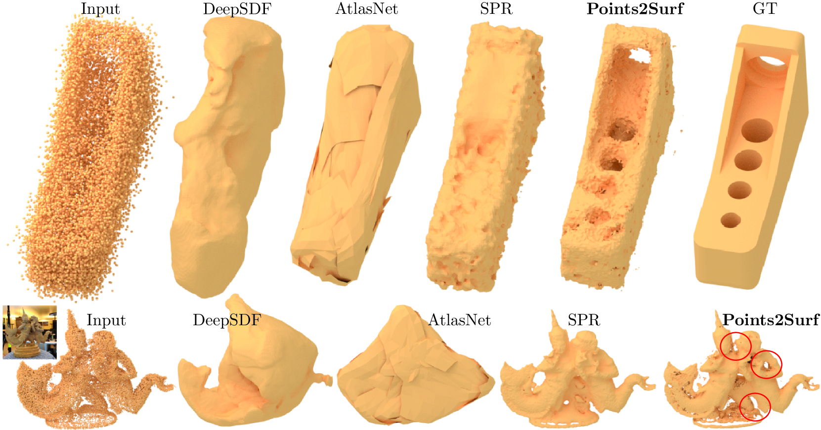
Figure 1: We present Points2Surf, a method to reconstruct an accurate implicit surface from a noisy point cloud. Unlike current data-driven surface reconstruction methods like DeepSDF and AtlasNet, it is patch-based, improves detail reconstruction, and unlike Screened Poisson Reconstruction (SPR), a learned prior of low-level patch shapes improves reconstruction accuracy. Note the quality of reconstructions, both geometric and topological, against the original surfaces. The ability of Points2Surf to generalize to new shapes makes it the first learning-based approach with significant generalization ability under both geometric and topological variations.

Converting unstructured point clouds to surfaces is a key step of most scanning-based asset creation workflows, including games and AR/VR applications. While scanning technologies have become more easily accessible (e.g., depth cameras on smart phones, portable scanners), algorithms for producing a surface mesh remain limited. A good surfacing algorithm should be able to handle raw point clouds with noisy and varying sampling density, work with different surface topologies, and generalize across a large range of scanned shapes.

Screened Poisson Reconstruction (SPR)[19] is the most commonly used method to convert an unstructured point cloud, along with its per-point normals, to a surface mesh. While the method is general, in absence of any data-priors, SPR typically produces smooth surfaces, can incorrectly close off holes and tunnels in noisy or non-uniformly sampled scans (see Figure1), and further degenerates when per-point normal estimates are erroneous.

Hence, several data-driven alternatives[21, 8, 30, 13] have recently been proposed. These methods specialize to particular object categories (e.g., cars, planes, chairs), and typically regress a global latent vector from any input scan. The networks can then decode a final shape (e.g., a collection of primitives[13] or a mesh[30]) from the estimated global latent vector. While such data-specific approaches handle noisy and partial scans, the methods do not generalize to new surfaces with varying shape and topology (see Figure1).

As a solution, we present Points2Surf, a method that learns to produce implicit surfaces directly from raw point clouds. During test time, our method can reliably handle raw scans to reproduce fine-scale data features even from noisy and non-uniformly sampled point sets, works for objects with varying topological attributes, and generalizes to new objects (see Figure1).

Our key insight is to decompose the problem into learning a global and a local function. For the global function, we learn the sign (i.e., inside or outside) of an implicit signed distance function, while, for the local function, we use a patch-based approach to learn absolute distance fields with respect to local point cloud patches. The global task is coarse (i.e., to learn the inside/outside of objects) and hence can be generalized across significant shape variations. The local task exploits the geometric observation that a large variety of shapes can be expressed in terms of a much smaller collection of atomic shape patches[2], which generalizes across arbitrary shapes. We demonstrate that such a factorization leads to a simple, robust, and generalizable approach to learn an implicit signed distance field, from which a final surface is extracted using Marching Cubes[23].

We test our algorithms on a range of synthetic and real examples, compare on unseen classes against both classical (reduction in reconstruction error by 30% over SPR) and learning based strong baselines (reduction in reconstruction error by 470% over DeepSDF[30] and 270% over AtlasNet[13]), and provide ablations studies. We consistently demonstrate both qualitative and quantitative improvement over all the methods that can be applied directly on raw scans.

2 Related Work

Several methods have been proposed to reconstruct surfaces from point clouds. We divide these into methods that aggregate information from a large dataset into a data-driven prior, and methods that do not use a data-driven prior.

Non-data-driven surface reconstruction.

Berger et al.[4] present an in-depth survey that is focused primarily on non-data-driven methods. Here we focus on approaches that are most relevant to our method. Scale space meshing[10] applies iterative mean curvature motion to smooth the points for meshing. It preserves multi-resolution features well. Ohrhallinger et al. propose a combinatorial method[27] which compares favorably with previous methods such as Wrap[11], TightCocone[9] and Shrink[5] especially for sparse sampling and thin structures. However, these methods are not designed to process noisy point clouds. Another line of work deforms initial meshes[33, 22] or parametric patches[36] to fit a noisy point cloud. These approaches however, cannot change the topology and connectivity of the original meshes or patches, usually resulting in a different connectivity or topology than the ground truth. The most widely-used approaches to reconstruct surfaces with arbitrary topology from noisy point clouds fit implicit functions to the point cloud and generate a surface as a level set of the function. Early work by Hoppe et al. introduced this approach[16], and since then several methods have focused on different representations of the implicit functions, like Fourier coefficients[17], wavelets[24], radial-basis functions[29] or multi-scale approaches[28, 26]. Alliez et al.[1] use a PCA of 3D Voronoi cells to estimate gradients and fit an implicit function by solving an eigenvalue problem. This approach tends to over-smooth geometric detail. Poisson reconstruction[18, 19] is the current gold standard for non-data-driven surface reconstruction from point clouds. None of the above methods make use of a prior that distills information about about typical surface shapes from a large dataset. Hence, while they are very general, they fail to handle partial and/or noisy input. We provide extensive comparisons to Screened Poisson Reconstruction (SPR)[19] in Section4.

Data-driven surface reconstruction.

Recently, several methods have been proposed to learn a prior of typical surface shapes from a large dataset. Early work was done by Sauerer et al.[21], where a decision tree is trained to predict the absolute distance part of an SDF, but ground truth normals are still required to obtain the sign (inside/outside) of the SDF. More recent data-driven methods represent surfaces with a single latent feature vector in a learned feature space. An encoder can be trained to obtain the feature vector from a point cloud. The feature representation acts as a strong prior, since only shapes that are representable in the feature space are reconstructed. Early methods use voxel-based representations of the surfaces, with spatial data-structures like octrees offsetting the cost of a full volumetric grid[34, 35]. Scan2Mesh[8] reconstructs a coarse mesh, including vertices and triangles, from a scan with impressive robustness to missing parts. However, the result is typically very coarse and not watertight or manifold, and does not apply to arbitrary new shapes. AtlasNet[13] uses multiple parametric surfaces as representation that jointly form a surface, achieving impressive accuracy and cross-category generalization. More recently, several approaches learn implicit function representations of surfaces[30, 6, 25]. These methods are trained to learn a functional that maps a latent encoding of a surface to an implicit function that can be used to extract a continuous surface. The implicit representation is more suitable for surfaces with complex topology and tends to produce aesthetically pleasing smooth surfaces.

The single latent feature vector that the methods above use to represent a surface acts as a strong prior, allowing these methods to reconstruct surfaces even in the presence of strong noise or missing parts; but it also limits the generality of these methods. The feature space typically captures only shapes that are similar to the shapes in the training set, and the variety of shapes that can be captured by the feature space is limited by the fixed capacity of the latent feature vector. Instead, we propose to decompose the SDF that is used to reconstruct the surface into a coarse global sign and a detailed local absolute distance. Separate feature vectors are used to represent the global and local parts, allowing us to represent detailed local geometry, without losing coarse global information about the shape.

3 Method

Our goal is to reconstruct a watertight surface S 𝑆 S italic_S from a 3D point cloud P={p 1,…,p N}𝑃 subscript 𝑝 1…subscript 𝑝 𝑁 P={p_{1},...,p_{N}}italic_P = { italic_p start_POSTSUBSCRIPT 1 end_POSTSUBSCRIPT , … , italic_p start_POSTSUBSCRIPT italic_N end_POSTSUBSCRIPT } that was sampled from the surface S 𝑆 S italic_S through a noisy sampling process, like a 3D scanner. We represent a surface as the zero-set of a Signed Distance Function (SDF) f S subscript 𝑓 𝑆 f_{S}italic_f start_POSTSUBSCRIPT italic_S end_POSTSUBSCRIPT:

S=L 0⁢(f S)={x∈ℝ 3|f S⁢(x)=0}.𝑆 subscript 𝐿 0 subscript 𝑓 𝑆 conditional-set 𝑥 superscript ℝ 3 subscript 𝑓 𝑆 𝑥 0 S=L_{0}(f_{S})={x\in\mathbb{R}^{3}\ |\ f_{S}(x)=0}.italic_S = italic_L start_POSTSUBSCRIPT 0 end_POSTSUBSCRIPT ( italic_f start_POSTSUBSCRIPT italic_S end_POSTSUBSCRIPT ) = { italic_x ∈ blackboard_R start_POSTSUPERSCRIPT 3 end_POSTSUPERSCRIPT | italic_f start_POSTSUBSCRIPT italic_S end_POSTSUBSCRIPT ( italic_x ) = 0 } .(1)

Recent work[30, 6, 25] has shown that such an implicit representation of the surface is particularly suitable for neural networks, which can be trained as functionals that take as input a latent representation of the point cloud and output an approximation of the SDF:

f S⁢(x)≈fP⁢(x)=s θ⁢(x|z),with⁢z=e ϕ⁢(P),formulae-sequence subscript 𝑓 𝑆 𝑥 subscript𝑓 𝑃 𝑥 subscript 𝑠 𝜃 conditional 𝑥 𝑧 with 𝑧 subscript 𝑒 italic-ϕ 𝑃 f_{S}(x)\approx\tilde{f}{P}(x)=s{\theta}(x|z),\ \text{with}\ z=e_{\phi}(P),italic_f start_POSTSUBSCRIPT italic_S end_POSTSUBSCRIPT ( italic_x ) ≈ over~ start_ARG italic_f end_ARG start_POSTSUBSCRIPT italic_P end_POSTSUBSCRIPT ( italic_x ) = italic_s start_POSTSUBSCRIPT italic_θ end_POSTSUBSCRIPT ( italic_x | italic_z ) , with italic_z = italic_e start_POSTSUBSCRIPT italic_ϕ end_POSTSUBSCRIPT ( italic_P ) ,(2)

where z 𝑧 z italic_z is a latent description of surface S 𝑆 S italic_S that can be encoded from the input point cloud with an encoder e 𝑒 e italic_e, and s 𝑠 s italic_s is implemented by a neural network that is conditioned on the latent vector z 𝑧 z italic_z. The networks s 𝑠 s italic_s and e 𝑒 e italic_e are parameterized by θ 𝜃\theta italic_θ and ϕ italic-ϕ\phi italic_ϕ, respectively. This representation of the surface is continuous, usually produces watertight meshes, and can naturally encode arbitrary topology. Different from non-data-driven methods like SPR[19], the trained network obtains a strong prior from the dataset it was trained on, that allows robust reconstruction of surfaces even from unreliable input, such as noisy and sparsely sampled point clouds. However, encoding the entire surface with a single latent vector imposes limitations on the accuracy and generality of the reconstruction, due to the limited capacity of the latent representation.

In this work, we factorize the SDF into the absolute distance f d superscript 𝑓 𝑑 f^{d}italic_f start_POSTSUPERSCRIPT italic_d end_POSTSUPERSCRIPT and the sign of the distance f s superscript 𝑓 𝑠 f^{s}italic_f start_POSTSUPERSCRIPT italic_s end_POSTSUPERSCRIPT, and take a closer look at the information needed to approximate each factor. To estimate the absolute distance fd⁢(x)superscript𝑓 𝑑 𝑥\tilde{f}^{d}(x)over~ start_ARG italic_f end_ARG start_POSTSUPERSCRIPT italic_d end_POSTSUPERSCRIPT ( italic_x ) at a query point x 𝑥 x italic_x, we only need a local neighborhood of the query point:

fP d⁢(x)=s θ d⁢(x|z x d),with⁢z x d=e ϕ d⁢(𝐩 x d),formulae-sequence superscript subscript𝑓 𝑃 𝑑 𝑥 subscript superscript 𝑠 𝑑 𝜃 conditional 𝑥 subscript superscript 𝑧 𝑑 𝑥 with subscript superscript 𝑧 𝑑 𝑥 subscript superscript 𝑒 𝑑 italic-ϕ subscript superscript 𝐩 𝑑 𝑥\tilde{f}{P}^{d}(x)=s^{d}{\theta}(x|z^{d}{x}),\ \text{with}\ z^{d}{x}=e^{d% }{\phi}(\mathbf{p}^{d}{x}),over~ start_ARG italic_f end_ARG start_POSTSUBSCRIPT italic_P end_POSTSUBSCRIPT start_POSTSUPERSCRIPT italic_d end_POSTSUPERSCRIPT ( italic_x ) = italic_s start_POSTSUPERSCRIPT italic_d end_POSTSUPERSCRIPT start_POSTSUBSCRIPT italic_θ end_POSTSUBSCRIPT ( italic_x | italic_z start_POSTSUPERSCRIPT italic_d end_POSTSUPERSCRIPT start_POSTSUBSCRIPT italic_x end_POSTSUBSCRIPT ) , with italic_z start_POSTSUPERSCRIPT italic_d end_POSTSUPERSCRIPT start_POSTSUBSCRIPT italic_x end_POSTSUBSCRIPT = italic_e start_POSTSUPERSCRIPT italic_d end_POSTSUPERSCRIPT start_POSTSUBSCRIPT italic_ϕ end_POSTSUBSCRIPT ( bold_p start_POSTSUPERSCRIPT italic_d end_POSTSUPERSCRIPT start_POSTSUBSCRIPT italic_x end_POSTSUBSCRIPT ) ,(3)

where 𝐩 x d⊂P subscript superscript 𝐩 𝑑 𝑥 𝑃\mathbf{p}^{d}{x}\subset P bold_p start_POSTSUPERSCRIPT italic_d end_POSTSUPERSCRIPT start_POSTSUBSCRIPT italic_x end_POSTSUBSCRIPT ⊂ italic_P is a local neighborhood of the point cloud centered around x 𝑥 x italic_x. Estimating the distance from an encoding of a local neighborhood gives us more accuracy than estimating it from an encoding of the entire shape, since the local encoding z x d subscript superscript 𝑧 𝑑 𝑥 z^{d}{x}italic_z start_POSTSUPERSCRIPT italic_d end_POSTSUPERSCRIPT start_POSTSUBSCRIPT italic_x end_POSTSUBSCRIPT can more accurately represent the local neighborhood around x 𝑥 x italic_x than the global encoding z 𝑧 z italic_z. Note that in a point cloud without noise and sufficiently dense sampling, the single closest point p⊂P superscript 𝑝 𝑃 p^{}\subset P italic_p start_POSTSUPERSCRIPT * end_POSTSUPERSCRIPT ⊂ italic_P to the query x 𝑥 x italic_x would be enough to obtain a good approximation of the absolute distance. But since we work with noisy and sparsely sampled point clouds, using a larger local neighborhood increases robustness.

In order to estimate the sign fs⁢(x)superscript𝑓 𝑠 𝑥\tilde{f}^{s}(x)over~ start_ARG italic_f end_ARG start_POSTSUPERSCRIPT italic_s end_POSTSUPERSCRIPT ( italic_x ) at the query point x 𝑥 x italic_x, we need global information about the entire shape, since the interior/exterior of a watertight surface cannot be estimated reliably from a local patch. Instead, we take a global sub-sample of the point cloud P 𝑃 P italic_P as input:

fP s⁢(x)=sgn⁢(gP s⁢(x))=sgn⁢(s θ s⁢(x|z x s)),with⁢z x s=e ψ s⁢(𝐩 x s),formulae-sequence superscript subscript𝑓 𝑃 𝑠 𝑥 sgn superscript subscript𝑔 𝑃 𝑠 𝑥 sgn subscript superscript 𝑠 𝑠 𝜃 conditional 𝑥 subscript superscript 𝑧 𝑠 𝑥 with subscript superscript 𝑧 𝑠 𝑥 subscript superscript 𝑒 𝑠 𝜓 subscript superscript 𝐩 𝑠 𝑥\tilde{f}{P}^{s}(x)=\mathrm{sgn}\big{(}\tilde{g}{P}^{s}(x)\big{)}=\mathrm{% sgn}\big{(}s^{s}{\theta}(x|z^{s}{x})\big{)},\ \text{with}\ z^{s}{x}=e^{s}{% \psi}(\mathbf{p}^{s}_{x}),over~ start_ARG italic_f end_ARG start_POSTSUBSCRIPT italic_P end_POSTSUBSCRIPT start_POSTSUPERSCRIPT italic_s end_POSTSUPERSCRIPT ( italic_x ) = roman_sgn ( over~ start_ARG italic_g end_ARG start_POSTSUBSCRIPT italic_P end_POSTSUBSCRIPT start_POSTSUPERSCRIPT italic_s end_POSTSUPERSCRIPT ( italic_x ) ) = roman_sgn ( italic_s start_POSTSUPERSCRIPT italic_s end_POSTSUPERSCRIPT start_POSTSUBSCRIPT italic_θ end_POSTSUBSCRIPT ( italic_x | italic_z start_POSTSUPERSCRIPT italic_s end_POSTSUPERSCRIPT start_POSTSUBSCRIPT italic_x end_POSTSUBSCRIPT ) ) , with italic_z start_POSTSUPERSCRIPT italic_s end_POSTSUPERSCRIPT start_POSTSUBSCRIPT italic_x end_POSTSUBSCRIPT = italic_e start_POSTSUPERSCRIPT italic_s end_POSTSUPERSCRIPT start_POSTSUBSCRIPT italic_ψ end_POSTSUBSCRIPT ( bold_p start_POSTSUPERSCRIPT italic_s end_POSTSUPERSCRIPT start_POSTSUBSCRIPT italic_x end_POSTSUBSCRIPT ) ,(4)

where 𝐩 x s⊂P subscript superscript 𝐩 𝑠 𝑥 𝑃\mathbf{p}^{s}{x}\subset P bold_p start_POSTSUPERSCRIPT italic_s end_POSTSUPERSCRIPT start_POSTSUBSCRIPT italic_x end_POSTSUBSCRIPT ⊂ italic_P is a global subsample of the point cloud, ψ 𝜓\psi italic_ψ are the parameters of the encoder, and gP s⁢(x)superscript subscript𝑔 𝑃 𝑠 𝑥\tilde{g}{P}^{s}(x)over~ start_ARG italic_g end_ARG start_POSTSUBSCRIPT italic_P end_POSTSUBSCRIPT start_POSTSUPERSCRIPT italic_s end_POSTSUPERSCRIPT ( italic_x ) are logits of the probability that x 𝑥 x italic_x has a positive sign. Working with logits avoids discontinuities near the surface, where the sign changes. Since it is more important to have accurate information closer to the query point, we sample 𝐩 x s subscript superscript 𝐩 𝑠 𝑥\mathbf{p}^{s}_{x}bold_p start_POSTSUPERSCRIPT italic_s end_POSTSUPERSCRIPT start_POSTSUBSCRIPT italic_x end_POSTSUBSCRIPT with a density gradient that is highest near the query point and falls off with distance from the query point.

We found that sharing information between the two latent descriptions z x s subscript superscript 𝑧 𝑠 𝑥 z^{s}{x}italic_z start_POSTSUPERSCRIPT italic_s end_POSTSUPERSCRIPT start_POSTSUBSCRIPT italic_x end_POSTSUBSCRIPT and z x d subscript superscript 𝑧 𝑑 𝑥 z^{d}{x}italic_z start_POSTSUPERSCRIPT italic_d end_POSTSUPERSCRIPT start_POSTSUBSCRIPT italic_x end_POSTSUBSCRIPT benefits both the absolute distance and the sign of the SDF, giving us the formulation we use in Points2Surf:

(fP d⁢(x),gP s⁢(x))=s θ⁢(x|z x d,z x s),with⁢z x d=e ϕ d⁢(𝐩 x d)⁢and⁢z x s=e ψ s⁢(𝐩 x s).formulae-sequence superscript subscript𝑓 𝑃 𝑑 𝑥 superscript subscript𝑔 𝑃 𝑠 𝑥 subscript 𝑠 𝜃 conditional 𝑥 subscript superscript 𝑧 𝑑 𝑥 subscript superscript 𝑧 𝑠 𝑥 with subscript superscript 𝑧 𝑑 𝑥 subscript superscript 𝑒 𝑑 italic-ϕ subscript superscript 𝐩 𝑑 𝑥 and subscript superscript 𝑧 𝑠 𝑥 subscript superscript 𝑒 𝑠 𝜓 subscript superscript 𝐩 𝑠 𝑥\big{(}\tilde{f}{P}^{d}(x),\tilde{g}{P}^{s}(x)\big{)}=s_{\theta}(x|z^{d}{x}% ,z^{s}{x}),\ \text{with}\ z^{d}{x}=e^{d}{\phi}(\mathbf{p}^{d}{x})\ \text{% and}\ z^{s}{x}=e^{s}{\psi}(\mathbf{p}^{s}{x}).( over~ start_ARG italic_f end_ARG start_POSTSUBSCRIPT italic_P end_POSTSUBSCRIPT start_POSTSUPERSCRIPT italic_d end_POSTSUPERSCRIPT ( italic_x ) , over~ start_ARG italic_g end_ARG start_POSTSUBSCRIPT italic_P end_POSTSUBSCRIPT start_POSTSUPERSCRIPT italic_s end_POSTSUPERSCRIPT ( italic_x ) ) = italic_s start_POSTSUBSCRIPT italic_θ end_POSTSUBSCRIPT ( italic_x | italic_z start_POSTSUPERSCRIPT italic_d end_POSTSUPERSCRIPT start_POSTSUBSCRIPT italic_x end_POSTSUBSCRIPT , italic_z start_POSTSUPERSCRIPT italic_s end_POSTSUPERSCRIPT start_POSTSUBSCRIPT italic_x end_POSTSUBSCRIPT ) , with italic_z start_POSTSUPERSCRIPT italic_d end_POSTSUPERSCRIPT start_POSTSUBSCRIPT italic_x end_POSTSUBSCRIPT = italic_e start_POSTSUPERSCRIPT italic_d end_POSTSUPERSCRIPT start_POSTSUBSCRIPT italic_ϕ end_POSTSUBSCRIPT ( bold_p start_POSTSUPERSCRIPT italic_d end_POSTSUPERSCRIPT start_POSTSUBSCRIPT italic_x end_POSTSUBSCRIPT ) and italic_z start_POSTSUPERSCRIPT italic_s end_POSTSUPERSCRIPT start_POSTSUBSCRIPT italic_x end_POSTSUBSCRIPT = italic_e start_POSTSUPERSCRIPT italic_s end_POSTSUPERSCRIPT start_POSTSUBSCRIPT italic_ψ end_POSTSUBSCRIPT ( bold_p start_POSTSUPERSCRIPT italic_s end_POSTSUPERSCRIPT start_POSTSUBSCRIPT italic_x end_POSTSUBSCRIPT ) .(5)

We describe the architecture of our encoders and decoder, the training setup, and our patch sampling strategy in more detail in Section3.1.

To reconstruct the surface S, we apply Marching Cubes[23] to a sample grid of the estimated SDF fd⁢(x)*fs⁢(x)superscript𝑓 𝑑 𝑥 superscript𝑓 𝑠 𝑥\tilde{f}^{d}(x)*\tilde{f}^{s}(x)over~ start_ARG italic_f end_ARG start_POSTSUPERSCRIPT italic_d end_POSTSUPERSCRIPT ( italic_x ) * over~ start_ARG italic_f end_ARG start_POSTSUPERSCRIPT italic_s end_POSTSUPERSCRIPT ( italic_x ). In Section3.2, we describe a strategy to improve performance by only evaluating a subset of the grid samples.

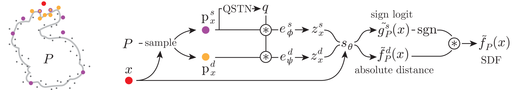
Figure 2: Points2Surf Architecture. Given a query point x 𝑥 x italic_x (red) and a point cloud P 𝑃 P italic_P (gray), we sample a local patch (yellow) and a coarse global subsample (purple) of the point cloud. These are encoded into two feature vectors that are fed to a decoder, which outputs a logit of the sign probability and the absolute distance of the SDF at the query point x 𝑥 x italic_x.

3.1 Architecture and Training

Figure2 shows an overview of our architecture. Our approach estimates the absolute distance fP d⁢(x)superscript subscript𝑓 𝑃 𝑑 𝑥\tilde{f}{P}^{d}(x)over~ start_ARG italic_f end_ARG start_POSTSUBSCRIPT italic_P end_POSTSUBSCRIPT start_POSTSUPERSCRIPT italic_d end_POSTSUPERSCRIPT ( italic_x ) and the sign logits gP s⁢(x)superscript subscript𝑔 𝑃 𝑠 𝑥\tilde{g}{P}^{s}(x)over~ start_ARG italic_g end_ARG start_POSTSUBSCRIPT italic_P end_POSTSUBSCRIPT start_POSTSUPERSCRIPT italic_s end_POSTSUPERSCRIPT ( italic_x ) at a query point based on two inputs: the query point x 𝑥 x italic_x and the point cloud P 𝑃 P italic_P.

Pointset sampling.

The local patch 𝐩 x d subscript superscript 𝐩 𝑑 𝑥\mathbf{p}^{d}{x}bold_p start_POSTSUPERSCRIPT italic_d end_POSTSUPERSCRIPT start_POSTSUBSCRIPT italic_x end_POSTSUBSCRIPT and the global sub-sample 𝐩 x s subscript superscript 𝐩 𝑠 𝑥\mathbf{p}^{s}{x}bold_p start_POSTSUPERSCRIPT italic_s end_POSTSUPERSCRIPT start_POSTSUBSCRIPT italic_x end_POSTSUBSCRIPT are both chosen from the point cloud P 𝑃 P italic_P based on the query point x 𝑥 x italic_x. The set 𝐩 x d subscript superscript 𝐩 𝑑 𝑥\mathbf{p}^{d}{x}bold_p start_POSTSUPERSCRIPT italic_d end_POSTSUPERSCRIPT start_POSTSUBSCRIPT italic_x end_POSTSUBSCRIPT is made of the n d subscript 𝑛 𝑑 n{d}italic_n start_POSTSUBSCRIPT italic_d end_POSTSUBSCRIPT nearest neighbors of the query point (we choose n d=300 subscript 𝑛 𝑑 300 n_{d}=300 italic_n start_POSTSUBSCRIPT italic_d end_POSTSUBSCRIPT = 300 but also experiment with other values). Unlike a fixed radius, the nearest neighbors are suitable for query points with arbitrary distance from the point cloud. The global sub-sample 𝐩 x s subscript superscript 𝐩 𝑠 𝑥\mathbf{p}^{s}_{x}bold_p start_POSTSUPERSCRIPT italic_s end_POSTSUPERSCRIPT start_POSTSUBSCRIPT italic_x end_POSTSUBSCRIPT is sampled from P 𝑃 P italic_P with a density gradient that decreases with distance from x 𝑥 x italic_x:

ρ⁢(p i)=v⁢(p i)∑p j∈P v⁢(p j),with⁢v⁢(p i)=[1−1.5⁢‖p i−x‖2 max p j∈P⁡‖p j−x‖2]0.05 1,formulae-sequence 𝜌 subscript 𝑝 𝑖 𝑣 subscript 𝑝 𝑖 subscript subscript 𝑝 𝑗 𝑃 𝑣 subscript 𝑝 𝑗 with 𝑣 subscript 𝑝 𝑖 superscript subscript delimited-[]1 1.5 subscript norm subscript 𝑝 𝑖 𝑥 2 subscript subscript 𝑝 𝑗 𝑃 subscript norm subscript 𝑝 𝑗 𝑥 2 0.05 1\rho(p_{i})=\frac{v(p_{i})}{\sum_{p_{j}\in P}v(p_{j})},\ \text{with}\ v(p_{i})% =\left[1-1.5\frac{|p_{i}-x|{2}}{\max{p_{j}\in P}|p_{j}-x|{2}}\right]{0% .05}^{1},italic_ρ ( italic_p start_POSTSUBSCRIPT italic_i end_POSTSUBSCRIPT ) = divide start_ARG italic_v ( italic_p start_POSTSUBSCRIPT italic_i end_POSTSUBSCRIPT ) end_ARG start_ARG ∑ start_POSTSUBSCRIPT italic_p start_POSTSUBSCRIPT italic_j end_POSTSUBSCRIPT ∈ italic_P end_POSTSUBSCRIPT italic_v ( italic_p start_POSTSUBSCRIPT italic_j end_POSTSUBSCRIPT ) end_ARG , with italic_v ( italic_p start_POSTSUBSCRIPT italic_i end_POSTSUBSCRIPT ) = [ 1 - 1.5 divide start_ARG ∥ italic_p start_POSTSUBSCRIPT italic_i end_POSTSUBSCRIPT - italic_x ∥ start_POSTSUBSCRIPT 2 end_POSTSUBSCRIPT end_ARG start_ARG roman_max start_POSTSUBSCRIPT italic_p start_POSTSUBSCRIPT italic_j end_POSTSUBSCRIPT ∈ italic_P end_POSTSUBSCRIPT ∥ italic_p start_POSTSUBSCRIPT italic_j end_POSTSUBSCRIPT - italic_x ∥ start_POSTSUBSCRIPT 2 end_POSTSUBSCRIPT end_ARG ] start_POSTSUBSCRIPT 0.05 end_POSTSUBSCRIPT start_POSTSUPERSCRIPT 1 end_POSTSUPERSCRIPT ,(6)

where ρ 𝜌\rho italic_ρ is the sample probability for a point p i∈P subscript 𝑝 𝑖 𝑃 p_{i}\in P italic_p start_POSTSUBSCRIPT italic_i end_POSTSUBSCRIPT ∈ italic_P, v 𝑣 v italic_v is the gradient that decreases with distance from x 𝑥 x italic_x, and the square brackets denote clamping. The minimum value for the clamping ensures that some far points are taken and the sub-sample can represent a closed object. We sample n s subscript 𝑛 𝑠 n_{s}italic_n start_POSTSUBSCRIPT italic_s end_POSTSUBSCRIPT points from P 𝑃 P italic_P according to this probability (we choose n s=1000 subscript 𝑛 𝑠 1000 n_{s}=1000 italic_n start_POSTSUBSCRIPT italic_s end_POSTSUBSCRIPT = 1000 in our experiments).

Pointset normalization.

Both 𝐩 x d subscript superscript 𝐩 𝑑 𝑥\mathbf{p}^{d}{x}bold_p start_POSTSUPERSCRIPT italic_d end_POSTSUPERSCRIPT start_POSTSUBSCRIPT italic_x end_POSTSUBSCRIPT and 𝐩 x s subscript superscript 𝐩 𝑠 𝑥\mathbf{p}^{s}{x}bold_p start_POSTSUPERSCRIPT italic_s end_POSTSUPERSCRIPT start_POSTSUBSCRIPT italic_x end_POSTSUBSCRIPT are normalized by centering them at the query point, and scaling them to unit radius. After running the network, the estimated distance is scaled back to the original size before comparing to the ground truth. Due to the centering, the query point is always at the origin of the normalized coordinate frame and does not need to be passed explicitly to the network. To normalize the orientation of both point subsets, we use a data-driven approach: a Quaternion Spatial Transformer Network (QSTN)[15] takes as input the global subset 𝐩 x s subscript superscript 𝐩 𝑠 𝑥\mathbf{p}^{s}_{x}bold_p start_POSTSUPERSCRIPT italic_s end_POSTSUPERSCRIPT start_POSTSUBSCRIPT italic_x end_POSTSUBSCRIPT and estimates a rotation represented as quaternion q 𝑞 q italic_q that is used to rotate both point subsets. We take the global subset as input, since the global information can help the network with finding a more consistent rotation. The QSTN is trained end-to-end with the full architecture, without direct supervision for the rotation.

Encoder and decoder architecture.

The local encoder e ϕ d subscript superscript 𝑒 𝑑 italic-ϕ e^{d}{\phi}italic_e start_POSTSUPERSCRIPT italic_d end_POSTSUPERSCRIPT start_POSTSUBSCRIPT italic_ϕ end_POSTSUBSCRIPT, and the global encoder e ψ s subscript superscript 𝑒 𝑠 𝜓 e^{s}{\psi}italic_e start_POSTSUPERSCRIPT italic_s end_POSTSUPERSCRIPT start_POSTSUBSCRIPT italic_ψ end_POSTSUBSCRIPT are both implemented as PointNets[31], sharing the same architecture, but not the parameters. Following the PointNet architecture, a feature representation for each point is computed using 5 5 5 5 MLP layers, with a spatial transformer in feature space after the third layer. Each layer except the last one uses batch normalization and ReLU. The point feature representations are then aggregated into point set feature representations z x d=e ϕ d⁢(𝐩 x d)subscript superscript 𝑧 𝑑 𝑥 subscript superscript 𝑒 𝑑 italic-ϕ subscript superscript 𝐩 𝑑 𝑥 z^{d}{x}=e^{d}{\phi}(\mathbf{p}^{d}{x})italic_z start_POSTSUPERSCRIPT italic_d end_POSTSUPERSCRIPT start_POSTSUBSCRIPT italic_x end_POSTSUBSCRIPT = italic_e start_POSTSUPERSCRIPT italic_d end_POSTSUPERSCRIPT start_POSTSUBSCRIPT italic_ϕ end_POSTSUBSCRIPT ( bold_p start_POSTSUPERSCRIPT italic_d end_POSTSUPERSCRIPT start_POSTSUBSCRIPT italic_x end_POSTSUBSCRIPT ) and z x s=e ψ s⁢(𝐩 x s)subscript superscript 𝑧 𝑠 𝑥 subscript superscript 𝑒 𝑠 𝜓 subscript superscript 𝐩 𝑠 𝑥 z^{s}{x}=e^{s}{\psi}(\mathbf{p}^{s}{x})italic_z start_POSTSUPERSCRIPT italic_s end_POSTSUPERSCRIPT start_POSTSUBSCRIPT italic_x end_POSTSUBSCRIPT = italic_e start_POSTSUPERSCRIPT italic_s end_POSTSUPERSCRIPT start_POSTSUBSCRIPT italic_ψ end_POSTSUBSCRIPT ( bold_p start_POSTSUPERSCRIPT italic_s end_POSTSUPERSCRIPT start_POSTSUBSCRIPT italic_x end_POSTSUBSCRIPT ) using a channel-wise maximum. The decoder s θ subscript 𝑠 𝜃 s_{\theta}italic_s start_POSTSUBSCRIPT italic_θ end_POSTSUBSCRIPT is implemented as 4-layer MLP that takes as input the concatenated feature vectors z x d subscript superscript 𝑧 𝑑 𝑥 z^{d}{x}italic_z start_POSTSUPERSCRIPT italic_d end_POSTSUPERSCRIPT start_POSTSUBSCRIPT italic_x end_POSTSUBSCRIPT and z x s subscript superscript 𝑧 𝑠 𝑥 z^{s}{x}italic_z start_POSTSUPERSCRIPT italic_s end_POSTSUPERSCRIPT start_POSTSUBSCRIPT italic_x end_POSTSUBSCRIPT and outputs both the absolute distance fd⁢(x)superscript𝑓 𝑑 𝑥\tilde{f}^{d}(x)over~ start_ARG italic_f end_ARG start_POSTSUPERSCRIPT italic_d end_POSTSUPERSCRIPT ( italic_x ) and sign logits gs⁢(x)superscript𝑔 𝑠 𝑥\tilde{g}^{s}(x)over~ start_ARG italic_g end_ARG start_POSTSUPERSCRIPT italic_s end_POSTSUPERSCRIPT ( italic_x ).

Losses and training.

We train our networks end-to-end to regress the absolute distance of the query point x 𝑥 x italic_x from the watertight ground-truth surface S 𝑆 S italic_S and classify the sign as positive (outside S 𝑆 S italic_S) or negative (inside S 𝑆 S italic_S). We assume that ground-truth surfaces are available during training for supervision. We use an L 2 subscript 𝐿 2 L_{2}italic_L start_POSTSUBSCRIPT 2 end_POSTSUBSCRIPT-based regression for the absolute distance:

ℒ d⁢(x,P,S)=‖tanh⁡(|fP d⁢(x)|)−tanh⁡(|d⁢(x,S)|)‖2 2,superscript ℒ 𝑑 𝑥 𝑃 𝑆 superscript subscript norm superscript subscript𝑓 𝑃 𝑑 𝑥 𝑑 𝑥 𝑆 2 2\mathcal{L}^{d}(x,P,S)=|\tanh(|\tilde{f}{P}^{d}(x)|)-\tanh(|d(x,S)|)|{2}^{% 2},caligraphic_L start_POSTSUPERSCRIPT italic_d end_POSTSUPERSCRIPT ( italic_x , italic_P , italic_S ) = ∥ roman_tanh ( | over~ start_ARG italic_f end_ARG start_POSTSUBSCRIPT italic_P end_POSTSUBSCRIPT start_POSTSUPERSCRIPT italic_d end_POSTSUPERSCRIPT ( italic_x ) | ) - roman_tanh ( | italic_d ( italic_x , italic_S ) | ) ∥ start_POSTSUBSCRIPT 2 end_POSTSUBSCRIPT start_POSTSUPERSCRIPT 2 end_POSTSUPERSCRIPT ,(7)

where d⁢(x,S)𝑑 𝑥 𝑆 d(x,S)italic_d ( italic_x , italic_S ) is the distance of x 𝑥 x italic_x to the ground-truth surface S 𝑆 S italic_S. The tanh\tanh roman_tanh function gives more weight to smaller absolute distances, which are more important for an accurate surface reconstruction. For the sign classification, we use the binary cross entropy H 𝐻 H italic_H as loss:

ℒ s⁢(x,P,S)=H⁢(σ⁢(gP s⁢(x)),[f S⁢(x)>0]),superscript ℒ 𝑠 𝑥 𝑃 𝑆 𝐻 𝜎 superscript subscript𝑔 𝑃 𝑠 𝑥 delimited-[]subscript 𝑓 𝑆 𝑥 0\mathcal{L}^{s}(x,P,S)=H\Big{(}\sigma\big{(}\tilde{g}{P}^{s}(x)\big{)},\ [f{% S}(x)>0]\Big{)},caligraphic_L start_POSTSUPERSCRIPT italic_s end_POSTSUPERSCRIPT ( italic_x , italic_P , italic_S ) = italic_H ( italic_σ ( over~ start_ARG italic_g end_ARG start_POSTSUBSCRIPT italic_P end_POSTSUBSCRIPT start_POSTSUPERSCRIPT italic_s end_POSTSUPERSCRIPT ( italic_x ) ) , [ italic_f start_POSTSUBSCRIPT italic_S end_POSTSUBSCRIPT ( italic_x ) > 0 ] ) ,(8)

where σ 𝜎\sigma italic_σ is the logistic function to convert the sign logits to probabilities, and [f S⁢(x)>0]delimited-[]subscript 𝑓 𝑆 𝑥 0[f_{S}(x)>0][ italic_f start_POSTSUBSCRIPT italic_S end_POSTSUBSCRIPT ( italic_x ) > 0 ] is 1 1 1 1 if x 𝑥 x italic_x is outside the surface S 𝑆 S italic_S and 0 0 otherwise. In our optimization, we minimize these two losses for all shapes and query points in the training set:

∑(P,S)∈𝒮∑x∈𝒳 S ℒ d⁢(x,P,S)+ℒ s⁢(x,P,S),subscript 𝑃 𝑆 𝒮 subscript 𝑥 subscript 𝒳 𝑆 superscript ℒ 𝑑 𝑥 𝑃 𝑆 superscript ℒ 𝑠 𝑥 𝑃 𝑆\sum_{(P,S)\in\mathcal{S}}\sum_{x\in\mathcal{X}_{S}}\mathcal{L}^{d}(x,P,S)+% \mathcal{L}^{s}(x,P,S),∑ start_POSTSUBSCRIPT ( italic_P , italic_S ) ∈ caligraphic_S end_POSTSUBSCRIPT ∑ start_POSTSUBSCRIPT italic_x ∈ caligraphic_X start_POSTSUBSCRIPT italic_S end_POSTSUBSCRIPT end_POSTSUBSCRIPT caligraphic_L start_POSTSUPERSCRIPT italic_d end_POSTSUPERSCRIPT ( italic_x , italic_P , italic_S ) + caligraphic_L start_POSTSUPERSCRIPT italic_s end_POSTSUPERSCRIPT ( italic_x , italic_P , italic_S ) ,(9)

where 𝒮 𝒮\mathcal{S}caligraphic_S is the set of surfaces S 𝑆 S italic_S and corresponding point clouds P 𝑃 P italic_P in the training set and 𝒳 S subscript 𝒳 𝑆\mathcal{X}_{S}caligraphic_X start_POSTSUBSCRIPT italic_S end_POSTSUBSCRIPT the set of query points for shape S 𝑆 S italic_S. Estimating the sign as a classification task instead of regressing the signed distance allows the network to express confidence through the magnitude of the sign logits, improving performance.

3.2 Surface Reconstruction

At inference time, we want to reconstruct a surface S~~𝑆\tilde{S}over~ start_ARG italic_S end_ARG from an estimated SDF f⁢(x)=fd⁢(x)*fs⁢(x)𝑓 𝑥 superscript𝑓 𝑑 𝑥 superscript𝑓 𝑠 𝑥\tilde{f}(x)=\tilde{f}^{d}(x)*\tilde{f}^{s}(x)over~ start_ARG italic_f end_ARG ( italic_x ) = over~ start_ARG italic_f end_ARG start_POSTSUPERSCRIPT italic_d end_POSTSUPERSCRIPT ( italic_x ) * over~ start_ARG italic_f end_ARG start_POSTSUPERSCRIPT italic_s end_POSTSUPERSCRIPT ( italic_x ). A straight-forward approach is to apply Marching Cubes[23] to a volumetric grid of SDF samples. Obtaining a high-resolution result, however, would require evaluating a prohibitive number of samples for each shape. We observe that in order to reconstruct a surface, a Truncated Signed Distance Field (TSDF) is sufficient, where the SDF is truncated to the interval [−ϵ,ϵ]italic-ϵ italic-ϵ[-\epsilon,\epsilon][ - italic_ϵ , italic_ϵ ] (we set ϵ italic-ϵ\epsilon italic_ϵ to three times the grid spacing in all our experiments). We only need to evaluate the SDF for samples that are inside this interval, while samples outside the interval merely need the correct sign. We leave samples with a distance larger than ϵ italic-ϵ\epsilon italic_ϵ to the nearest point in P 𝑃 P italic_P blank, and in a second step, we propagate the signed distance values from non-blank to blank samples, to obtain the correct sign in the truncated regions of the TSDF. We iteratively apply a box filter of size 3 3 superscript 3 3 3^{3}3 start_POSTSUPERSCRIPT 3 end_POSTSUPERSCRIPT at the blank samples until convergence. In each step, we update initially unknown samples only if the filter response is greater than a user-defined confidence threshold (we use 13 in our experiments). After each step, the samples are set to -1 if the filter response was negative or to +1 for a positive response.

4 Results

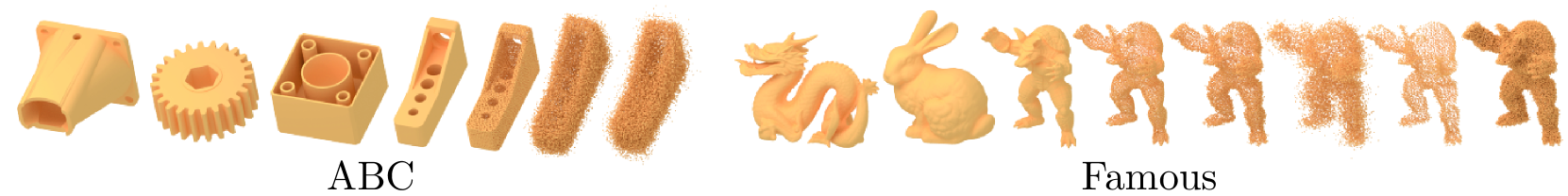
Figure 3: Dataset examples. Examples of the ABC dataset and its three variants are shown on the left, examples of the famous dataset and its five variants on the right.

Table 1: Comparison of reconstruction errors. We show the Chamfer distance between reconstructed and ground-truth surfaces averaged over all shapes in a dataset. Both the absolute value of the error multiplied by 100 100 100 100 (abs.), and the error relative to Point2Surf (rel.) are shown to facilitate the comparison. Our method consistently performs better than the baselines, due to its strong and generalizable prior.

Table 2: Quantitative comparison of reconstruction errors on the Thingi10k dataset. Note that none of the methods was retrained on the Thingi10k in order to test generalization to new data.

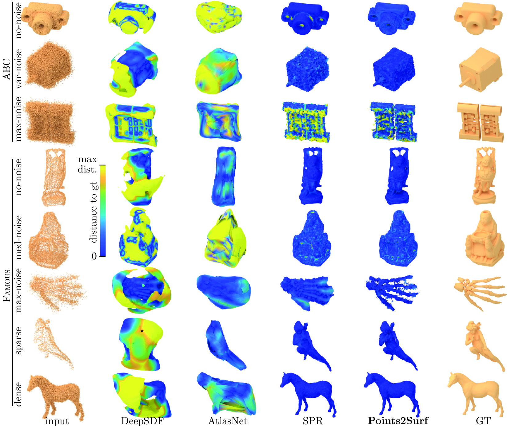
Figure 4: Qualitative comparison of surface reconstructions. We evaluate one example from each dataset variant with each method. Colors show the distance of the reconstructed surface to the ground-truth surface.

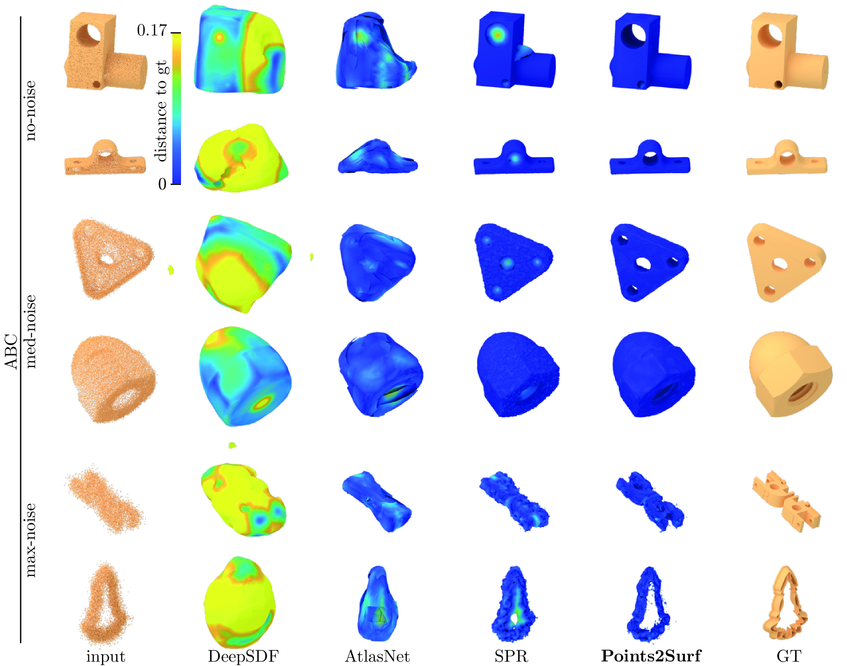
Figure 5: Additional qualitative comparison of surface reconstructions on the ABC dataset. We evaluate two examples from each dataset variant with each method. Colors show the distance of the reconstructed surface to the ground truth surface.

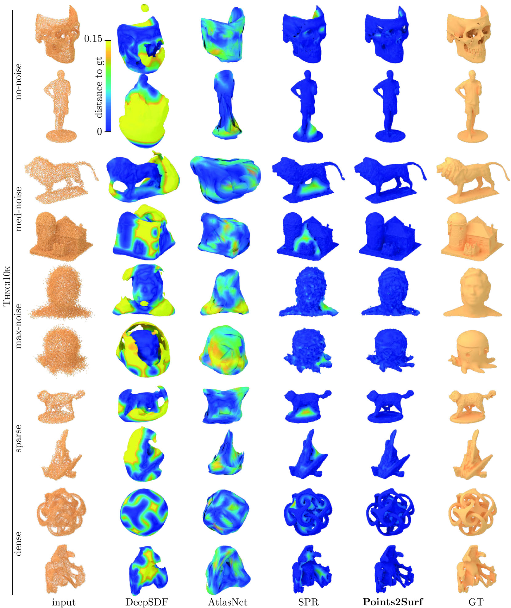
Figure 6: Qualitative comparison of surface reconstructions on the Thingi10k dataset. We evaluate two examples from each dataset variant with each method. Colors show the distance of the reconstructed surface to the ground truth surface, shades of blue indicating low error.

We compare our method to SPR as the gold standard for non-data-driven surface reconstruction and to two state-of-the-art data-driven surface reconstruction methods. We provide both qualitative and quantitative comparisons on several datasets in Section4.2, perform an ablation study in Section4.3, and provide detailed timings in Section4.4

4.1 Datasets

We train and evaluate on the ABC dataset[20] which contains a large number and variety of high-quality CAD meshes. We pick 4950 4950 4950 4950 clean watertight meshes for training and 100 100 100 100 meshes for the validation and test sets. Note that each mesh produces a large number of diverse patches as training samples. Operating on local patches also allows us to generalize better, which we demonstrate on two additional test-only datasets: a dataset of 22 22 22 22 diverse meshes which are well-known in geometry processing, such as the Utah teapot and the Stanford Bunny, which we call the Famous dataset, and 3 3 3 3 Real scans of complex objects used in several denoising papers[37, 32]. Examples from each dataset are shown in Figure3. The ABC dataset contains predominantly CAD models of mechanical parts, while the Famous dataset contains more organic shapes, such as characters and animals. Since we train on the ABC dataset, the Famous dataset serves to test the generalizability of our method versus baselines.

Pointcloud sampling.

As a pre-processing step, we center all meshes at the origin and scale them uniformly to fit within the unit cube. To obtain point clouds P 𝑃 P italic_P from the meshes S 𝑆 S italic_S in the datasets, we simulate scanning them with a time-of-flight sensor from random viewpoints using BlenSor[14]. BlenSor realistically simulates various types of scanner noise and artifacts such as backfolding, ray reflections, and per-ray noise. We scan each mesh in the Famous dataset with 10 10 10 10 scans and each mesh in the ABC dataset with a random number of scans, between 5 5 5 5 and 30 30 30 30. For each scan, we place the scanner at a random location on a sphere centered at the origin, with the radius chosen randomly in U⁢[3⁢L,5⁢L]𝑈 3 𝐿 5 𝐿 U[3L,5L]italic_U [ 3 italic_L , 5 italic_L ], where L 𝐿 L italic_L is the largest side of the mesh bounding box. The scanner is oriented to point at a location with small random offset from the origin, between U⁢[−0.1⁢L,0.1⁢L]𝑈 0.1 𝐿 0.1 𝐿 U[-0.1L,0.1L]italic_U [ - 0.1 italic_L , 0.1 italic_L ] along each axis, and rotated randomly around the view direction. Each scan has a resolution of 176×144 176 144 176\times 144 176 × 144, resulting in roughly 25 25 25 25 k points, minus some points missing due to simulated scanning artifacts. The point clouds of multiple scans of a mesh are merged to obtain the final point cloud.

Dataset variants.

We create multiple versions of both the ABC and Famous datasets, with varying amount of per-ray noise. This Gaussian noise added to the depth values simulates inaccuracies in the depth measurements. For both datasets, we create a noise-free version of the point clouds, called ABC no-noise and Famous no-noise. Also, we make versions with strong noise (standard deviation is 0.05⁢L 0.05 𝐿 0.05L 0.05 italic_L) called ABC max-noise and Famous max-noise. Since we need varying noise strength for the training, we create a version of ABC where the standard deviation is randomly chosen in U⁢[0,0.05⁢L]𝑈 0 0.05 𝐿 U[0,0.05L]italic_U [ 0 , 0.05 italic_L ] (ABC var-noise), and a version with a constant noise strength of 0.01⁢L 0.01 𝐿 0.01L 0.01 italic_L for the test set (Famous med-noise). Additionally we create sparser (5 5 5 5 scans) and denser (30 30 30 30 scans) point clouds in comparison to the 10 10 10 10 scans of the other variants of Famous. Both variants have a medium noise strength of 0.01⁢L 0.01 𝐿 0.01L 0.01 italic_L. Additionally, we show a comparison with scanned objects from the Thingi10k dataset using the same variants as Famous. We take 100 meshes that are tagged with ‘scan’ or ‘sculpture’. These objects are mostly animals, humans and faces, many of them realistic, some artistic. The training set uses the ABC var-noise version, all other variants are used for evaluation only.

Query points.

The training set also contains a set 𝒳 S subscript 𝒳 𝑆\mathcal{X}_{S}caligraphic_X start_POSTSUBSCRIPT italic_S end_POSTSUBSCRIPT of query points for each (point cloud, mesh) pair (P,S)∈𝒮 𝑃 𝑆 𝒮(P,S)\in\mathcal{S}( italic_P , italic_S ) ∈ caligraphic_S. Query points closer to the surface are more important for the surface reconstruction and more difficult to estimate. Hence, we randomly sample a set of 1000 1000 1000 1000 points on the surface and offset them in the normal direction by a uniform random amount in U⁢[−0.02⁢L,0.02⁢L]𝑈 0.02 𝐿 0.02 𝐿 U[-0.02L,0.02L]italic_U [ - 0.02 italic_L , 0.02 italic_L ]. An additional 1000 1000 1000 1000 query points are sampled randomly in the unit cube that contains the surface, for a total of 2000 2000 2000 2000 query points per mesh. During training, we randomly sample a subset of 1000 1000 1000 1000 query points per mesh in each epoch.

4.2 Comparison to Baselines

We compare our method to recent data-driven surface reconstruction methods, AtlasNet[13] and DeepSDF[30], and to SPR[19], which is still the gold standard in non-data-driven surface reconstruction from point clouds. Both AtlasNet and DeepSDF represent a full surface as a single latent vector that is decoded into either a set of parametric surface patches in AtlasNet, or an SDF in DeepSDF. In contrast, SPR solves for an SDF that has a given sparse set of point normals as gradients, and takes on values of 0 0 at the point locations. We use the default values and training protocols given by the authors for all baselines (more details in the Supplementary) and re-train the two data-driven methods on our training set. We provide SPR with point normals as input, which we estimate from the input point cloud using the recent PCPNet[15].

For DeepSDF, we followed the method in the original paper with minor adaptations. For the training set, we take our query points and the corresponding Signed Distances (SD) as GT SDF samples. For the test sets, we take the point clouds from our dataset. For each point, we generate 2 SDF samples, one in positive and one in negative normal direction, with random offset. The normals are taken from the ground truth face closest to the sample. The corresponding SDs are the +- normal offset. We add 20% random samples from the unit cube with GT SD.

Error metric.

To measure the reconstruction error of each method, we sample both the reconstructed surface and the ground-truth surface with 10 10 10 10 k points and compute the Chamfer distance[3, 12] between the two point sets:

d ch⁢(A,B):=1|A|⁢∑p i∈A min p j∈B⁡‖p i−p j‖2 2+1|B|⁢∑p j∈B min p i∈A⁡‖p j−p i‖2 2,assign subscript 𝑑 ch 𝐴 𝐵 1 𝐴 subscript subscript 𝑝 𝑖 𝐴 subscript subscript 𝑝 𝑗 𝐵 subscript superscript norm subscript 𝑝 𝑖 subscript 𝑝 𝑗 2 2 1 𝐵 subscript subscript 𝑝 𝑗 𝐵 subscript subscript 𝑝 𝑖 𝐴 subscript superscript norm subscript 𝑝 𝑗 subscript 𝑝 𝑖 2 2 d_{\text{ch}}(A,B):=\frac{1}{|A|}\sum_{p_{i}\in A}\min_{p_{j}\in B}|p_{i}-p_{% j}|^{2}{2}\ +\frac{1}{|B|}\sum{p_{j}\in B}\min_{p_{i}\in A}|p_{j}-p_{i}|^% {2}_{2},italic_d start_POSTSUBSCRIPT ch end_POSTSUBSCRIPT ( italic_A , italic_B ) := divide start_ARG 1 end_ARG start_ARG | italic_A | end_ARG ∑ start_POSTSUBSCRIPT italic_p start_POSTSUBSCRIPT italic_i end_POSTSUBSCRIPT ∈ italic_A end_POSTSUBSCRIPT roman_min start_POSTSUBSCRIPT italic_p start_POSTSUBSCRIPT italic_j end_POSTSUBSCRIPT ∈ italic_B end_POSTSUBSCRIPT ∥ italic_p start_POSTSUBSCRIPT italic_i end_POSTSUBSCRIPT - italic_p start_POSTSUBSCRIPT italic_j end_POSTSUBSCRIPT ∥ start_POSTSUPERSCRIPT 2 end_POSTSUPERSCRIPT start_POSTSUBSCRIPT 2 end_POSTSUBSCRIPT + divide start_ARG 1 end_ARG start_ARG | italic_B | end_ARG ∑ start_POSTSUBSCRIPT italic_p start_POSTSUBSCRIPT italic_j end_POSTSUBSCRIPT ∈ italic_B end_POSTSUBSCRIPT roman_min start_POSTSUBSCRIPT italic_p start_POSTSUBSCRIPT italic_i end_POSTSUBSCRIPT ∈ italic_A end_POSTSUBSCRIPT ∥ italic_p start_POSTSUBSCRIPT italic_j end_POSTSUBSCRIPT - italic_p start_POSTSUBSCRIPT italic_i end_POSTSUBSCRIPT ∥ start_POSTSUPERSCRIPT 2 end_POSTSUPERSCRIPT start_POSTSUBSCRIPT 2 end_POSTSUBSCRIPT ,(10)

where A 𝐴 A italic_A and B 𝐵 B italic_B are point sets sampled on the two surfaces. The Chamfer distance penalizes both false negatives (missing parts) and false positives (excess parts).

Quantitative and qualitative comparison.

A quantitative comparison of the reconstruction quality is shown in Tables1 and2. Figures4,5 and6 compare a few reconstructions qualitatively. All methods were trained on the training set of the ABC var-noise dataset, which contains predominantly mechanical parts, while the more organic shapes in the Famous dataset test how well each method can generalize to novel types of shapes.

Both DeepSDF and AtlasNet use a global shape prior, which is well suited for a dataset with high geometric consistency among the shapes, like cars in ShapeNet, but struggles with the significantly larger geometric and topological diversity in our datasets, reflected in a higher reconstruction error than SPR or Points2Surf. This is also clearly visible in Figure4, where the surfaces reconstructed by DeepSDF and AtlasNet appear over-smoothed and inaccurate.

In SPR, the full shape space does not need to be encoded into a prior with limited capacity, resulting in a better accuracy. But this lack of a strong prior also prevents SPR from robustly reconstructing typical surface features, such as holes or planar patches (see Figures1 and 4).

Points2Surf learns a prior of local surface details, instead of a prior for global surface shapes. This local prior helps recover surface details like holes and planar patches more robustly, improving our accuracy over SPR. Since there is less variety and more consistency in local surface details compared to global surface shapes, our method generalizes better and achieves a higher accuracy than the data-driven methods that use a prior over the global surface shape.

Generalization.

A comparison of our generalization performance against AtlasNet and DeepSDF shows an advantage for our method. In Table1, we can see that the error for DeepSDF and AtlasNet increases more when going from the ABC dataset to the Famous dataset than the error for our method. This suggests that our method generalizes better from the CAD models in the ABC dataset set to the more organic shapes in the Famous dataset.

Figure 7: Comparison of reconstruction details. Our learned prior improves the reconstruction robustness for geometric detail compared to SPR.

Topological Quality.

Figure7 shows examples of geometric detail that benefits from our prior. The first example shows that small features such as holes can be recovered from a very weak geometric signal in a noisy point cloud. Concavities, such as the space between the legs of the Armadillo, and fine shape details like the Armadillo’s hand are also recovered more accurately in the presence of strong noise. In the heart example, the concavity makes it hard to estimate the correct normal direction based on only a local neighborhood, which causes SPR to produce artifacts. In contrast, the global information we use in our patches helps us estimate the correct sign, even if the local neighborhood is misleading.

Effect of Noise.

Examples of reconstructions from point clouds with increasing amounts of noise are shown in Figure8. Our learned prior for local patches and our coarse global surface information makes it easier to find small holes and large concavities. In the medium noise setting, we can recover the small holes and the large concavity of the surface. With maximum noise, it is very difficult to detect the small holes, but we can still recover the concavity.

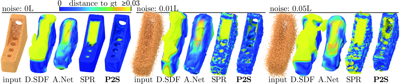
Figure 8: Effect of noise on our reconstruction. DeepSDF (D.SDF), AtlasNet (A.Net), SPR and Point2Surf (P2S) are applied to increasingly noisy point clouds. Our patch-based data-driven approach is more accurate than DeepSDF and AtlasNet, and can more robustly recover small holes and concavities than SPR.

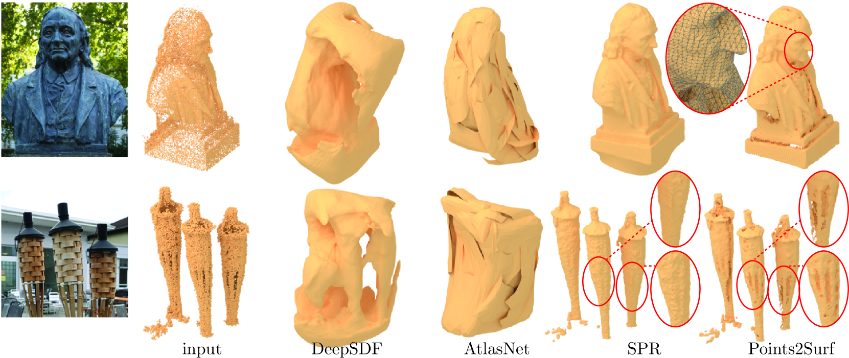
Figure 9: Reconstruction of real-world point clouds. Snapshots of the real-world objects are shown on the left. DeepSDF and AtlasNet do not generalize well, resulting in inaccurate reconstructions, while the smoothness prior of SPR results in loss of detail near concavities and holes. Our data-driven local prior better preserves these details.

Real-world data.

The real-world point clouds in Figure1 bottom and Figure9 bottom both originate from a multi-view dataset[37] and were obtained with a plane-sweep algorithm[7] from multiple photographs of an object. We additionally remove outliers using the recent PointCleanNet[32]. Figure9 top was obtained by the authors through an SfM approach. DeepSDF and AtlasNet do not generalize well to unseen shape categories. SPR performs significantly better but its smoothness prior tends to over-smooth shapes and close holes. Points2Surf better preserves holes and details, at the cost of a slight increase in topological noise. Our technique also generalizes to unseen point-cloud acquisition methods.

4.3 Ablation Study

We evaluate several design choices in (e vanilla subscript 𝑒 vanilla e_{\text{vanilla}}italic_e start_POSTSUBSCRIPT vanilla end_POSTSUBSCRIPT) using an ablation study, as shown in Table3. We evaluate the number of nearest neighbors k=300 𝑘 300 k=300 italic_k = 300 that form the local patch by decreasing and increasing k 𝑘 k italic_k by a factor of 4 4 4 4 (k small subscript 𝑘 small k_{\text{small}}italic_k start_POSTSUBSCRIPT small end_POSTSUBSCRIPT and k large subscript 𝑘 large k_{\text{large}}italic_k start_POSTSUBSCRIPT large end_POSTSUBSCRIPT), effectively halving and doubling the size of the local patch. A large k 𝑘 k italic_k performs significantly worse because we lose local detail with a larger patch size. A small k 𝑘 k italic_k still works reasonably well, but gives a lower performance, especially with strong noise. We also test a fixed radius for the local patch, with three different sizes (r small:=0.05⁢L assign subscript 𝑟 small 0.05 𝐿 r_{\text{small}}:=0.05L italic_r start_POSTSUBSCRIPT small end_POSTSUBSCRIPT := 0.05 italic_L, r med:=0.1⁢L assign subscript 𝑟 med 0.1 𝐿 r_{\text{med}}:=0.1L italic_r start_POSTSUBSCRIPT med end_POSTSUBSCRIPT := 0.1 italic_L and r large:=0.2⁢L assign subscript 𝑟 large 0.2 𝐿 r_{\text{large}}:=0.2L italic_r start_POSTSUBSCRIPT large end_POSTSUBSCRIPT := 0.2 italic_L). A fixed patch size is less suitable than nearest neighbors when computing the distance at query points that are far away from the surface, giving a lower performance than the standard nearest neighbor setting. The next variant is using a single shared encoder (e shared subscript 𝑒 shared e_{\text{shared}}italic_e start_POSTSUBSCRIPT shared end_POSTSUBSCRIPT) for both the global sub-sample 𝐩 x s subscript superscript 𝐩 𝑠 𝑥\mathbf{p}^{s}{x}bold_p start_POSTSUPERSCRIPT italic_s end_POSTSUPERSCRIPT start_POSTSUBSCRIPT italic_x end_POSTSUBSCRIPT and the local patch 𝐩 x d subscript superscript 𝐩 𝑑 𝑥\mathbf{p}^{d}{x}bold_p start_POSTSUPERSCRIPT italic_d end_POSTSUPERSCRIPT start_POSTSUBSCRIPT italic_x end_POSTSUBSCRIPT, by concatenating the two before encoding them. The performance of e shared subscript 𝑒 shared e_{\text{shared}}italic_e start_POSTSUBSCRIPT shared end_POSTSUBSCRIPT is competitive, but shows that using two separate encoders increases performance. Omitting the QSTN (e no_QSTN subscript 𝑒 no_QSTN e_{\text{no_QSTN}}italic_e start_POSTSUBSCRIPT no_QSTN end_POSTSUBSCRIPT) speeds-up the training by roughly 10% and yields slightly better results. The reason is probably that our outputs are rotation-invariant in contrast to the normals of PCPNet. Using a uniform global sub-sample in e uniform subscript 𝑒 uniform e_{\text{uniform}}italic_e start_POSTSUBSCRIPT uniform end_POSTSUBSCRIPT increases the quality over the distance-dependent sub-sampling in e vanilla subscript 𝑒 vanilla e_{\text{vanilla}}italic_e start_POSTSUBSCRIPT vanilla end_POSTSUBSCRIPT. This uniform sub-sample preserves more information about the far side of the object, which benefits the inside/outside classification. Due to resource constraints, we trained all models in Table3 for 50 epochs only. For applications where speed, memory and simplicity is important, we recommend using a shared encoder without the QSTN and with uniform sub-sampling.

Table 3: Ablation Study. We compare Points2Surf (e vanilla subscript 𝑒 vanilla e_{\text{vanilla}}italic_e start_POSTSUBSCRIPT vanilla end_POSTSUBSCRIPT) to several variants and show the Chamfer distance relative to Points2Surf. Please see the text for details.

4.4 Timings

We compare the wall-clock times of Points2Surf vanilla to the baselines. Because AtlasNet is very fast, we show the mean of 3 runs. We take the times of reconstructing the 100 shapes of the ABC med-noise test set using 16 worker processes. With this, we can show a fair comparison that takes parallelization, loading times and different bottlenecks into account. We ran the timings on a consumer-grade PC with a Ryzen 7 3600X, 64 GB DDR4 RAM and a GTX 1070. The mean times per shape in seconds are: Points2Surf 712.1, DeepSDF 199.5, SPR 157.5, AtlasNet 0.1. Since DeepSDF and SPR need normals, we included 156.5 seconds for the normal estimation using PCPNet.

The heuristic and sign propagation allows us to reduce the number of inferred query points to 1.67% of a full grid in ABC var-noise. Assuming linear scaling, the inference time is reduced from almost 12 hours to 11.5 minutes. This speed-up comes at the cost of 19.2 seconds per shape. The heuristic is less efficient with noise. For the ABC no-noise, the number of query points is reduced to 0.77% and for ABC max-noise to 2.33%.

We trained a smaller version of e uniform subscript 𝑒 uniform e_{\text{uniform}}italic_e start_POSTSUBSCRIPT uniform end_POSTSUBSCRIPT with only about 15% parameters. The mini version reduces the reconstruction time by roughly 68% compared to e vanilla subscript 𝑒 vanilla e_{\text{vanilla}}italic_e start_POSTSUBSCRIPT vanilla end_POSTSUBSCRIPT (from 11.5 to 3.7 minutes per mesh), at the cost of an increase in the reconstruction error of roughly 55% on ABC var-noise (Chamfer distance from 150.6 for e vanilla subscript 𝑒 vanilla e_{\text{vanilla}}italic_e start_POSTSUBSCRIPT vanilla end_POSTSUBSCRIPT to 234.3 for the small version of e uniform subscript 𝑒 uniform e_{\text{uniform}}italic_e start_POSTSUBSCRIPT uniform end_POSTSUBSCRIPT).

5 Conclusion

We have presented Points2Surf as a method for surface reconstruction from raw point clouds. Our method reliably captures both geometric and topological details, and generalizes to unseen shapes more robustly than current methods.

The distance-dependent global sub-sample may cause inconsistencies between the outputs of neighboring patches, which results in bumpy surfaces.

One interesting future direction would be to perform multi-scale reconstructions, where coarser levels provide consistency for finer levels, reducing the bumpiness. This should also decrease the computation times significantly. Finally, it would be interesting to develop a differentiable version of Marching Cubes to jointly train SDF estimation and surface extraction.

6 Acknowledgements

This work has been supported by the FWF projects no. P24600, P27972 and P32418 and the ERC Starting Grant SmartGeometry (StG-2013-335373).

References

• [1] Alliez, P., Cohen-Steiner, D., Tong, Y., Desbrun, M.: Voronoi-based variational reconstruction of unoriented point sets. In: Symposium on Geometry processing. vol.7, pp. 39–48 (2007)
• [2] Badki, A., Gallo, O., Kautz, J., Sen, P.: Meshlet priors for 3d mesh reconstruction. ArXiv (2020)
• [3] Barrow, H.G., Tenenbaum, J.M., Bolles, R.C., Wolf, H.C.: Parametric correspondence and chamfer matching: Two new techniques for image matching. In: Proceedings of the 5th International Joint Conference on Artificial Intelligence - Volume 2. pp. 659–663. IJCAI’77, Morgan Kaufmann Publishers Inc., San Francisco, CA, USA (1977)
• [4] Berger, M., Tagliasacchi, A., Seversky, L.M., Alliez, P., Guennebaud, G., Levine, J.A., Sharf, A., Silva, C.T.: A survey of surface reconstruction from point clouds. In: Computer Graphics Forum. vol.36, pp. 301–329. Wiley Online Library (2017)
• [5] Chaine, R.: A geometric convection approach of 3-d reconstruction. In: Proceedings of the 2003 Eurographics/ACM SIGGRAPH symposium on Geometry processing. pp. 218–229. Eurographics Association (2003)
• [6] Chen, Z., Zhang, H.: Learning implicit fields for generative shape modeling. In: Proc.of CVPR (2019)
• [7] Collins, R.T.: A space-sweep approach to true multi-image matching. In: Proceedings CVPR IEEE Computer Society Conference on Computer Vision and Pattern Recognition. pp. 358–363. IEEE (1996)
• [8] Dai, A., Nießner, M.: Scan2mesh: From unstructured range scans to 3d meshes. In: Proc. Computer Vision and Pattern Recognition (CVPR), IEEE (2019)
• [9] Dey, T.K., Goswami, S.: Tight cocone: a water-tight surface reconstructor. In: Proceedings of the eighth ACM symposium on Solid modeling and applications. pp. 127–134. ACM (2003)
• [10] Digne, J., Morel, J.M., Souzani, C.M., Lartigue, C.: Scale space meshing of raw data point sets. In: Computer Graphics Forum. vol.30, pp. 1630–1642. Wiley Online Library (2011)
• [11] Edelsbrunner, H.: Surface reconstruction by wrapping finite sets in space. In: Discrete and computational geometry, pp. 379–404. Springer (2003)
• [12] Fan, H., Su, H., Guibas, L.J.: A point set generation network for 3d object reconstruction from a single image. In: Proceedings of the IEEE conference on computer vision and pattern recognition. pp. 605–613 (2017)
• [13] Groueix, T., Fisher, M., Kim, V.G., Russell, B., Aubry, M.: AtlasNet: A Papier-Mâché Approach to Learning 3D Surface Generation. In: Proceedings IEEE Conf. on Computer Vision and Pattern Recognition (CVPR) (2018)
• [14] Gschwandtner, M., Kwitt, R., Uhl, A., Pree, W.: Blensor: Blender sensor simulation toolbox. In: International Symposium on Visual Computing. pp. 199–208. Springer (2011)
• [15] Guerrero, P., Kleiman, Y., Ovsjanikov, M., Mitra, N.J.: PCPNet: Learning local shape properties from raw point clouds. Computer Graphics Forum 37(2), 75–85 (2018)
• [16] Hoppe, H., DeRose, T., Duchamp, T., McDonald, J., Stuetzle, W.: Surface reconstruction from unorganized points, vol.26. ACM (1992)
• [17] Kazhdan, M.: Reconstruction of solid models from oriented point sets. In: Proceedings of the third Eurographics symposium on Geometry processing. p.73. Eurographics Association (2005)
• [18] Kazhdan, M., Bolitho, M., Hoppe, H.: Poisson surface reconstruction. In: Proc.of the Eurographics symposium on Geometry processing (2006)
• [19] Kazhdan, M., Hoppe, H.: Screened poisson surface reconstruction. ACM Transactions on Graphics (ToG) 32(3), 29 (2013)
• [20] Koch, S., Matveev, A., Jiang, Z., Williams, F., Artemov, A., Burnaev, E., Alexa, M., Zorin, D., Panozzo, D.: Abc: A big cad model dataset for geometric deep learning. In: The IEEE Conference on Computer Vision and Pattern Recognition (CVPR) (June 2019)
• [21] Ladicky, L., Saurer, O., Jeong, S., Maninchedda, F., Pollefeys, M.: From point clouds to mesh using regression. In: Proceedings of the IEEE International Conference on Computer Vision. pp. 3893–3902 (2017)
• [22] Li, G., Liu, L., Zheng, H., Mitra, N.J.: Analysis, reconstruction and manipulation using arterial snakes. In: ACM SIGGRAPH Asia 2010 Papers. SIGGRAPH ASIA ’10, Association for Computing Machinery, New York, NY, USA (2010)
• [23] Lorensen, W.E., Cline, H.E.: Marching cubes: A high resolution 3d surface construction algorithm. In: ACM siggraph computer graphics. vol.21, pp. 163–169. ACM (1987)
• [24] Manson, J., Petrova, G., Schaefer, S.: Streaming surface reconstruction using wavelets. In: Computer Graphics Forum. vol.27, pp. 1411–1420. Wiley Online Library (2008)
• [25]Mescheder, L., Oechsle, M., Niemeyer, M., Nowozin, S., Geiger, A.: Occupancy networks: Learning 3d reconstruction in function space. In: Proc.of CVPR (2019)
• [26] Nagai, Y., Ohtake, Y., Suzuki, H.: Smoothing of partition of unity implicit surfaces for noise robust surface reconstruction. In: Computer Graphics Forum. vol.28, pp. 1339–1348. Wiley Online Library (2009)
• [27] Ohrhallinger, S., Mudur, S., Wimmer, M.: Minimizing edge length to connect sparsely sampled unstructured point sets. Computers & Graphics 37(6), 645–658 (2013)
• [28] Ohtake, Y., Belyaev, A., Seidel, H.P.: A multi-scale approach to 3d scattered data interpolation with compactly supported basis functions. In: 2003 Shape Modeling International. pp. 153–161. IEEE (2003)
• [29] Ohtake, Y., Belyaev, A., Seidel, H.P.: 3d scattered data interpolation and approximation with multilevel compactly supported rbfs. Graphical Models 67(3), 150–165 (2005)
• [30]Park, J.J., Florence, P., Straub, J., Newcombe, R., Lovegrove, S.: Deepsdf: Learning continuous signed distance functions for shape representation. arXiv preprint arXiv:1901.05103 (2019)
• [31] Qi, C.R., Su, H., Mo, K., Guibas, L.J.: Pointnet: Deep learning on point sets for 3d classification and segmentation. arXiv preprint arXiv:1612.00593 (2016)
• [32] Rakotosaona, M.J., La Barbera, V., Guerrero, P., Mitra, N.J., Ovsjanikov, M.: Pointcleannet: Learning to denoise and remove outliers from dense point clouds. Computer Graphics Forum (2019)
• [33] Sharf, A., Lewiner, T., Shamir, A., Kobbelt, L., Cohen-Or, D.: Competing fronts for coarse–to–fine surface reconstruction. In: Computer Graphics Forum. vol.25, pp. 389–398. Wiley Online Library (2006)
• [34] Tatarchenko, M., Dosovitskiy, A., Brox, T.: Octree generating networks: Efficient convolutional architectures for high-resolution 3d outputs. In: Proceedings of the IEEE International Conference on Computer Vision. pp. 2088–2096 (2017)
• [35] Wang, P.S., Sun, C.Y., Liu, Y., Tong, X.: Adaptive o-cnn: A patch-based deep representation of 3d shapes. ACM Transactions on Graphics (TOG) 37(6), 1–11 (2018)
• [36] Williams, F., Schneider, T., Silva, C.T., Zorin, D., Bruna, J., Panozzo, D.: Deep geometric prior for surface reconstruction. In: Proceedings of the IEEE Conference on Computer Vision and Pattern Recognition. pp. 10130–10139 (2019)
• [37] Wolff, K., Kim, C., Zimmer, H., Schroers, C., Botsch, M., Sorkine-Hornung, O., Sorkine-Hornung, A.: Point cloud noise and outlier removal for image-based 3d reconstruction. In: 2016 Fourth International Conference on 3D Vision (3DV). pp. 118–127 (Oct 2016)