143 kB

Title: FBNetV5: Neural Architecture Search for Multiple Tasks in One Run

URL Source: https://arxiv.org/html/2111.10007

Markdown Content: Bichen Wu 1, Chaojian Li 2∗†, Hang Zhang 1, Xiaoliang Dai 1, Peizhao Zhang 1,

Matthew Yu 1, Jialiang Wang 1, Yingyan Lin 2, Peter Vajda 1

1 Meta Reality Labs, 2 Rice University

{wbc,zhanghang,xiaoliangdai,stzpz,mattcyu,jialiangw,vajdap}@fb.com

{cl114,yingyan.lin}@rice.edu

Abstract

Neural Architecture Search (NAS) has been widely adopted to design accurate and efficient image classification models. However, applying NAS to a new computer vision task still requires a huge amount of effort. This is because 1) previous NAS research has been over-prioritized on image classification while largely ignoring other tasks; 2) many NAS works focus on optimizing task-specific components that cannot be favorably transferred to other tasks; and 3) existing NAS methods are typically designed to be “proxyless” and require significant effort to be integrated with each new task’s training pipelines. To tackle these challenges, we propose FBNetV5, a NAS framework that can search for neural architectures for a variety of vision tasks with much reduced computational cost and human effort. Specifically, we design 1) a search space that is simple yet inclusive and transferable; 2) a multitask search process that is disentangled with target tasks’ training pipeline; and 3) an algorithm to simultaneously search for architectures for multiple tasks with a computational cost agnostic to the number of tasks. We evaluate the proposed FBNetV5 targeting three fundamental vision tasks – image classification, object detection, and semantic segmentation. Models searched by FBNetV5 in a single run of search have outperformed the previous state-of-the-art in all the three tasks: image classification (e.g., ↑↑\uparrow↑1.3% ImageNet top-1 accuracy under the same FLOPs as compared to FBNetV3), semantic segmentation (e.g., ↑↑\uparrow↑1.8% higher ADE20K val. mIoU than SegFormer with 3.6×\times× fewer FLOPs), and object detection (e.g., ↑↑\uparrow↑1.1% COCO val. mAP with 1.2×\times× fewer FLOPs as compared to YOLOX).

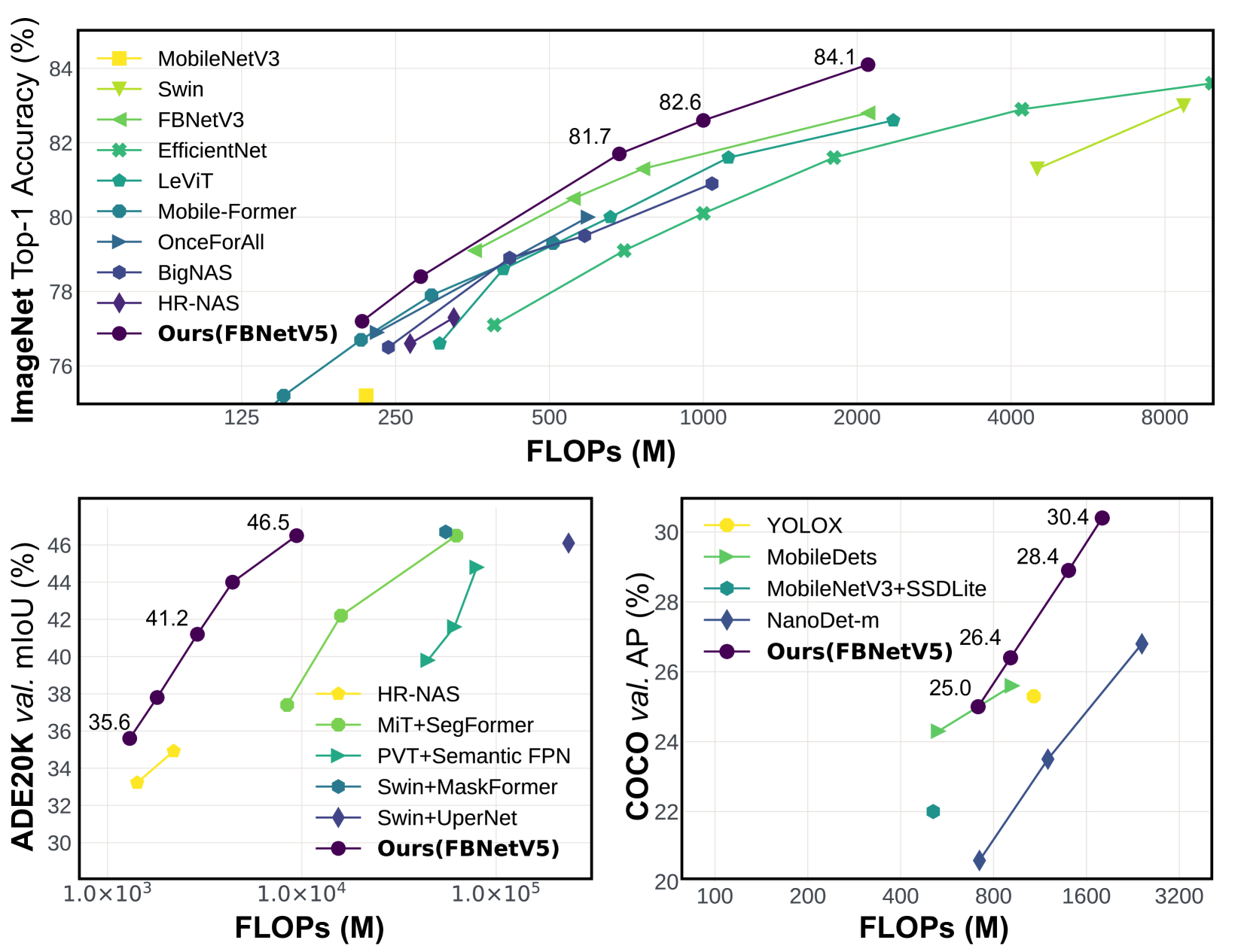
Figure 1: The architectures simultaneously searched in a single run of FBNetV5 outperforms the SotA performance in three tasks: ImageNet[15] image classification, ADE20K[65] semantic segmentation, and COCO[32] object detection.

1 Introduction

Recent breakthroughs in deep neural networks (DNNs) have fueled a growing demand for deploying DNNs in perception systems for a wide range of computer vision (CV) applications that are powered by various fundamental CV tasks, including classification, object detection, and semantic segmentation. To develop real-world DNN based perception systems, the neural architecture design is among the most important factors that determine the achievable task performance and efficiency. Nevertheless, designing neural architectures for different applications is challenging due to its prohibitive computational cost, intractable design space[40, 17, 12], diverse application-driven deployment requirements[57, 29, 61], and so on.

To tackle the aforementioned challenges, the CV community has been exploring neural architecture search (NAS) to design DNNs for CV tasks. In general, the expectations for NAS are two-fold: First, to build better neural architectures with stronger performance and higher efficiency; and second, to automate the design process in order to reduce the human effort and computational cost for DNN design. While the former ensures effective real-world solutions, the latter is critical to facilitate the fast development of DNNs to more applications. Looking back at the progress of recent years, it is fair to say that NAS has met the first expectation in advancing the frontiers of accuracy and efficiency, especially for image classification tasks. However, existing NAS methods still fall short of meeting the second expectation.

The reasons for the above limitation include the following. First, over the years the NAS community has been over fixated on benchmarking NAS methods on image classification tasks, driven by the commonly believed assumption that the best models for image classification are also the best backbones for other tasks. However, this assumption is not always true[61, 18, 9, 64], and often leads to suboptimal architectures for many non-classification tasks. Second, many existing NAS works focus on optimizing task-specific components that are not transferable or favorable to other tasks. For example, [46] only searches for the encoder part within the encoder-decoder structure of segmentation tasks, while the optimal encoder is coupled with the decoder designs. [20] is customized to RetinaNet[31] in object detection tasks. As a result, NAS advances made for one task do not necessarily favor other tasks or help reduce the design effort. Finally, a popular belief in current NAS practice is that it is better for NAS to be “proxyless” and a NAS method should be integrated into the target tasks’ training pipeline for directly optimizing the corresponding architectures based on the training losses of each target task[3, 4, 63]. However, this makes NAS unscalable when dealing with many new tasks, since adding each new task would require nontrivial efforts to integrate the NAS techniques into the existing training pipeline of the target task. In particular, many popular NAS methods conduct search by training a supernet[63, 3, 53], adding dedicated cost regularization to the loss function[16], adopting special initialization[63], and so on. These techniques often heavily interfere with the target task’s training process and thus requires much engineering effort to re-tune the hyperparameters to achieve the desired performance.

In this work, we propose FBNetV5, a NAS framework, that can simultaneously search for backbone topologies for multiple tasks in a single run of search. As a proof of concept, we target three fundamental computer vision tasks – image classification, object detection, and semantic segmentation. Starting from a state-of-the-art image classification model, i.e., FBNetV3 [13], we construct a supernet consisting of parallel paths with multiple resolutions, similar to HRNet[54, 16]. Based on the supernet, FBNetV5 searches for the optimal topology for each target task by parameterizing a set of binary masks indicating whether to keep or drop a building block in the supernet. To disentangle the search process from the target tasks’ training pipeline, we conduct search by training the supernet on a proxy multitask dataset with classification, object detection, and semantic segmentation labels. Following [21], the dataset is based on ImageNet, with detection and segmentation labels generated by pretrained open-source models. To make the computational cost and hyper-parameter tuning effort agnostic to the number of tasks, we propose a supernet training algorithm that simultaneously search for task architectures in one run. After the supernet training, we individually train the searched task-specific architectures to uncover their performance.

Excitingly, in addition to requiring reduced computational cost and human effort, extensive experiments show that FBNetV5 produces compact models that can achieve SotA performance on all three target tasks. On ImageNet [15] classification, our model achieved 1.3 1.3 1.3 1.3% higher top-1 accuracy under the same FLOPs as compared to FBNetV3 [13]; on ADE20K[65] semantic segmentation, our model achieved 1.8 1.8 1.8 1.8% higher mIoU than SegFormer [60] with 3.6×\times× fewer FLOPs; on COCO [32] object detection, our model achieved 1.1% higher mAP with 1.2×\times× fewer FLOPs compared to YOLOX [19]. It is worth noting that all our well-performing architectures are searched simultaneously in a single run, yet they beat the SotA neural architectures that are delicately searched or designed for each task.

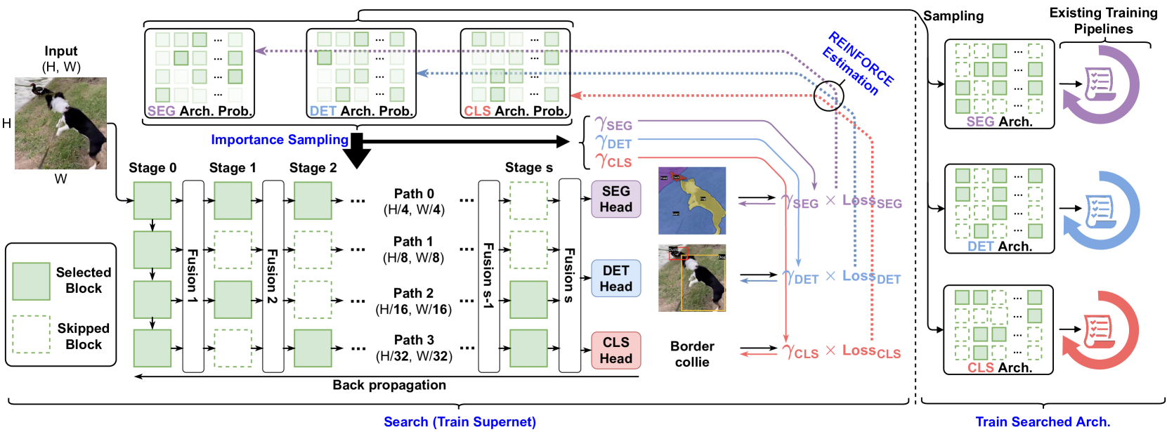
Figure 2: Overview of FBNetV5. We search backbone topologies for multiple tasks by training a supernet once on a multitask dataset. Each task has its own architecture distribution from which we sample task-specific architectures and train them using the existing training pipeline of the target tasks. Supernet configurations in Appendix A. Fusion module details in AppendixB. Search process in Algorithm 4.

2 Related Works

Neural Architecture Search for Efficient DNNs. Various NAS methods have been developed to design efficient DNNs, aiming to 1) achieve boosted accuracy vs. efficiency trade-offs[23, 45, 25] and 2) automate the design process to reduce human effort and computational cost. Early NAS works mostly adopt reinforcement learning[67, 47] or evolutionary search algorithms[42] which require substantial resources. To reduce the search cost, differentiable NAS[57, 52, 4, 8, 33] was developed to differentiably update the weights and architectures. Recently, to deliver multiple neural architectures meeting different cost constraints,[3, 63] propose to jointly train all the sub-networks in a weight-sharing supernet and then locate the optimal architectures under different cost constraints without re-training or fine-tuning. However, unlike our work, all the works above focus on a single task, mostly image classification, and they do not reduce the effort of designing architectures for other tasks.

Task-aware Neural Architecture Design. To facilitate designing optimal DNNs for various tasks, recent works [24, 35, 54] propose to design general architecture backbones for different CV tasks. In parallel, with the belief that each CV task requires its own unique architecture to achieve the task-specific optimal accuracy vs. efficiency trade-off,[46, 7, 20, 31, 50] develop dedicated search spaces for different CV tasks, from which they search for task-aware DNN architectures. However, these existing methods mostly focus on optimizing task-specific components of which the advantages are not transferable to other tasks. Recent works [16, 11] begin to focus on designing networks for multiple tasks in a unified search space and has shown promising results. However, they are designed to be “proxyless” and the search process needs to be integrated to downstream tasks’s training pipeline. This makes it less scalable to add new tasks, since it requires non-trivial engineering effort and compute cost to integrate NAS to the existing training pipeline of a target task. Our work bypasses this by using a disentangled search process, and we conduct search for multiple tasks in one run. This is computationally efficient and allows us to utilize target tasks’ existing training pipelines with no extra efforts.

3 Method

In this section, we present our proposed FBNetV5 framework that aims to reduce the computational cost and human effort required by NAS for multiple tasks. FBNetV5 contains three key components: 1) A simple yet inclusive and transferable search space (Section 3.1); 2) A search process equipped with a multitask learning proxy to disentangle NAS from target tasks’ training pipelines (Section 3.2); and 3) a search algorithm to simultaneously produce architectures for multiple tasks at a constant computational cost agnostic to the number of target tasks (Section 3.3).

3.1 Search Space

To search for architectures for multiple tasks, we design the search space to meet three standards: 1) Simple and elegant: we favor simple search space over complicated ones; 2) Inclusive: the search space should include strong architectures for all target tasks; and 3) Transferable: the searched architectures should be useful not only for one model, but also transferable to a family of models.

Inspired by HRNet[54, 16], we extend a SotA classification model, FBNetV3[13], to a supernet with parallel paths and multiple stages. Each path has a different resolution while blocks on the same path have the same resolution. This is shown in Figure2 (bottom-left). We divide an FBNetV3 into 4 partitions along the depth dimension, each partition outputs a feature map with a resolution down-sampled by 4 4 4 4, 8 8 8 8, 16 16 16 16, and 32 32 32 32 times, respectively. Stage 0 of the supernet is essentially the FBNetV3 model. For following stages, we use the last 2 layers of each partition to construct a block per stage. During inference, we first compute Stage 0 of the supernet, and then compute the remaining blocks by topological order. Similar to [54], we insert (lightweight) fusion modules (see AppendixB) between stages to fuse information from different paths (resolutions). A block-wise model configuration of the supernet can be found in Appendix A.

The aforementioned supernet contains blocks with varying significance to different tasks. By conventional wisdom, a classification architecture may only need blocks on the low-resolution paths, while segmentation or object detection would favor blocks with a higher resolution. Based on this, we search for network topologies, i.e., which blocks to select or skip for different tasks. Formally, for a supernet with P 𝑃 P italic_P paths, S 𝑆 S italic_S stages, and B=S×P 𝐵 𝑆 𝑃 B=S\times P italic_B = italic_S × italic_P blocks, a candidate architecture can be characterized by a binary vector 𝐚∈{0,1}B 𝐚 superscript 0 1 𝐵\mathbf{a}\in{0,1}^{B}bold_a ∈ { 0 , 1 } start_POSTSUPERSCRIPT italic_B end_POSTSUPERSCRIPT, where 𝐚 i=1 subscript 𝐚 𝑖 1\mathbf{a}{i}=1 bold_a start_POSTSUBSCRIPT italic_i end_POSTSUBSCRIPT = 1 means to select block-i 𝑖 i italic_i and 𝐚 i=0 subscript 𝐚 𝑖 0\mathbf{a}{i}=0 bold_a start_POSTSUBSCRIPT italic_i end_POSTSUBSCRIPT = 0 means to skip and remove the corresponding connections from and to this block. More details about the implementation of fusion modules with skipped blocks are provided in AppendixB.

We believe that this search space is simple and elegant. It only contains binary choices for each of the B 𝐵 B italic_B blocks. This is much simpler than other search space design that considers how to mix different types of operators (convolutions and transformers) together, or how to wire operators with complicated connections. Furthermore, the search space is inclusive. As a sanity check, the search space include most of the mainstream network topologies for CV tasks, e.g., 1) the simple linear topology for most of the classification models, 2) the U-Net [44] and PANet [34] topology for semantic segmentation, and 3) the Feature-Pyramid Networks (FPN) [30] and BiFPN [50] for object detection, as illustrated in AppendixC. The searched architecture topology is transferable. FBNet contains a series of models from small to large. We conduct search on a FBNet-A based supernet, and the topology can be transferred to other models. It is worth noting that transferring topology to models of different sizes, depths, and resolutions is also a common practice adopted by works such as FPN [30] and BiFPN [50]).

3.2 Disentangled Search Process

A popular belief is that NAS should be proxyless and the search process should be integrated into each target task’s training pipeline for achieving better results. However, implementing and integrating the search process to each target task’s pipeline can require significant engineering effort. Moreover, many NAS techniques heavily interfere with the target task’s training and thus requires much engineering effort to re-tune the hyperparameters.

To avoid the above limitations, we design a search process that is disentangled with target tasks’ training pipeline. Specifically, we conduct search by training a supernet on a multitask dataset where each image is annotated with labels from all target tasks. Following [57], the supernet training jointly optimize the model weights and more importantly, task-specific architecture distributions (e.g., the SEG, DET, and CLS Arch. Prob. in Figure2). The goal of the search process is to obtain a task-specific architecture distribution from which we can sample architectures for the target tasks. The searched models can then be trained using the existing training pipeline of the target tasks without the necessity of implementing the search process into the tasks’ training pipeline or re-tune the existing hyper-parameters. The search process is shown in Figure 2.

As there is no large-scale multitask dataset publicly available, we follow [21] to construct a pseudo-labeled dataset based on ImageNet. Specifically, we use 1) original ImageNet labels for classification, 2) open-source CenterNet2 [66] pretrained on the COCO object detection dataset to generate pseudo detection labels, and 3) open-source MaskFormer [10] pretrained on the COCO-stuff semantic segmentation dataset (171 classes) to generate pixel-wise segmentation labels. In addition, we follow [21] to filter out object detection results with a confidence lower than 0.5, and set segmentation predictions whose maximum probability lower than 0.5 to be the “don’t-care” category. As such, this dataset can easily extend to include more tasks by using open-source pretrained models to generate task-specific pseudo labels.

3.3 Search Algorithm

Our search algorithm is based on the differentiable neural architecture search [33, 57, 52] for low computational cost compared with other methods, such as sampling-based methods [13, 48]. For multiple tasks, a simple idea is to apply the conventional single-task NAS (Algorithm1) T 𝑇 T italic_T times for each task. To make this more scalable, we derive a novel search algorithm with a constant computational cost agnostic to the number of tasks (Algorithm4). For better clarity, We introduce the derivation of the search algorithm in four steps corresponding to Algorithm1, 2, 3, and 4, respectively. We summarize and compare the four search algorithms at each step in Table 1. We visualize Algorithm 4 in Figure 2.

Table 1: Summary of the differentiable NAS algorithms. T 𝑇 T italic_T represents the number of tasks.

Search Algorithms#Tasks to Handle Search Cost #Forward#Backprop. Per Iter Per Iter Algorithm11 1 1 Algorithm2T 𝑇 T italic_T T 𝑇 T italic_T T 𝑇 T italic_T Algorithm3T 𝑇 T italic_T 1 T 𝑇 T italic_T Algorithm4T 𝑇 T italic_T 1 1

3.3.1 Differentiable NAS for a Single Task

We start from a typical differentiable NAS designed for a single task, which can be formulated as

min 𝐚∈𝒜,𝐰⁢ℓ t⁢(𝐚,𝐰),𝐚 𝒜 𝐰 superscript ℓ 𝑡 𝐚 𝐰\underset{\mathbf{a}\in\mathcal{A},\mathbf{w}}{\min}~{}\ell^{t}(\mathbf{a},% \mathbf{w}),start_UNDERACCENT bold_a ∈ caligraphic_A , bold_w end_UNDERACCENT start_ARG roman_min end_ARG roman_ℓ start_POSTSUPERSCRIPT italic_t end_POSTSUPERSCRIPT ( bold_a , bold_w ) ,(1)

where 𝐚 𝐚\mathbf{a}bold_a is a candidate architecture in the search space 𝒜 𝒜\mathcal{A}caligraphic_A, 𝐰 𝐰\mathbf{w}bold_w is the supernet’s weight, and ℓ t⁢(⋅)superscript ℓ 𝑡⋅\ell^{t}(\cdot)roman_ℓ start_POSTSUPERSCRIPT italic_t end_POSTSUPERSCRIPT ( ⋅ ) is the loss function of task-t 𝑡 t italic_t that also considers the cost of architecture 𝐚 𝐚\mathbf{a}bold_a. Following [57, 14], the cost of an architecture can be defined in terms of FLOPs, parameter size, latency, energy, etc.

In our work, we search in a block-level search space. For block-b 𝑏 b italic_b of the supernet, we have

𝐲=a b⁢f b⁢(𝐱)+(1−a b)⁢𝐱,𝐲 subscript 𝑎 𝑏 subscript 𝑓 𝑏 𝐱 1 subscript 𝑎 𝑏 𝐱\mathbf{y}=a_{b}f_{b}(\mathbf{x})+(1-a_{b})\mathbf{x},bold_y = italic_a start_POSTSUBSCRIPT italic_b end_POSTSUBSCRIPT italic_f start_POSTSUBSCRIPT italic_b end_POSTSUBSCRIPT ( bold_x ) + ( 1 - italic_a start_POSTSUBSCRIPT italic_b end_POSTSUBSCRIPT ) bold_x ,(2)

where 𝐱 𝐱\mathbf{x}bold_x, 𝐲 𝐲\mathbf{y}bold_y are input and output of block-b 𝑏 b italic_b function f b⁢(⋅)subscript 𝑓 𝑏⋅f_{b}(\cdot)italic_f start_POSTSUBSCRIPT italic_b end_POSTSUBSCRIPT ( ⋅ ). a b∈{0,1}subscript 𝑎 𝑏 0 1 a_{b}\in{0,1}italic_a start_POSTSUBSCRIPT italic_b end_POSTSUBSCRIPT ∈ { 0 , 1 } is a binary variable that determines whether to compute block-b 𝑏 b italic_b or skip it. Under this setting, the search space 𝒜={0,1}B 𝒜 superscript 0 1 𝐵\mathcal{A}={0,1}^{B}caligraphic_A = { 0 , 1 } start_POSTSUPERSCRIPT italic_B end_POSTSUPERSCRIPT for Equation (1) is combinatorial and contains 2 B superscript 2 𝐵 2^{B}2 start_POSTSUPERSCRIPT italic_B end_POSTSUPERSCRIPT candidates, where B 𝐵 B italic_B is the number of blocks. To solve it efficiently, we relax the problem as

min 𝝅,𝐰⁢𝔼 𝐚∼p 𝝅⁢{ℓ t⁢(𝐚,𝐰)},𝝅 𝐰 subscript 𝔼 similar-to 𝐚 subscript 𝑝 𝝅 superscript ℓ 𝑡 𝐚 𝐰\underset{{\bm{\pi}},\mathbf{w}}{\min}~{}\mathbb{E}{\mathbf{a}\sim p{{\bm{% \pi}}}}{\ell^{t}(\mathbf{a},\mathbf{w})},start_UNDERACCENT bold_italic_π , bold_w end_UNDERACCENT start_ARG roman_min end_ARG blackboard_E start_POSTSUBSCRIPT bold_a ∼ italic_p start_POSTSUBSCRIPT bold_italic_π end_POSTSUBSCRIPT end_POSTSUBSCRIPT { roman_ℓ start_POSTSUPERSCRIPT italic_t end_POSTSUPERSCRIPT ( bold_a , bold_w ) } ,(3)

where 𝐚∈{0,1}B 𝐚 superscript 0 1 𝐵\mathbf{a}\in{0,1}^{B}bold_a ∈ { 0 , 1 } start_POSTSUPERSCRIPT italic_B end_POSTSUPERSCRIPT is a random variable sampled from a distribution p 𝝅 subscript 𝑝 𝝅 p_{\bm{\pi}}italic_p start_POSTSUBSCRIPT bold_italic_π end_POSTSUBSCRIPT, parameterized by 𝝅∈[0,1]B 𝝅 superscript 0 1 𝐵{\bm{\pi}}\in[0,1]^{B}bold_italic_π ∈ [ 0 , 1 ] start_POSTSUPERSCRIPT italic_B end_POSTSUPERSCRIPT. For each block, we independently sample a b∼Bernoulli⁢(π b)similar-to subscript 𝑎 𝑏 Bernoulli subscript 𝜋 𝑏 a_{b}\sim\text{Bernoulli}(\pi_{b})italic_a start_POSTSUBSCRIPT italic_b end_POSTSUBSCRIPT ∼ Bernoulli ( italic_π start_POSTSUBSCRIPT italic_b end_POSTSUBSCRIPT ) from a Bernoulli distribution with an expected value of π b subscript 𝜋 𝑏\pi_{b}italic_π start_POSTSUBSCRIPT italic_b end_POSTSUBSCRIPT. The probability of architecture 𝐚 𝐚\mathbf{a}bold_a computes as

p 𝝅⁢(𝐚)=∏b=1 B π b a b⁢(1−π b)(1−a b).subscript 𝑝 𝝅 𝐚 superscript subscript product 𝑏 1 𝐵 superscript subscript 𝜋 𝑏 subscript 𝑎 𝑏 superscript 1 subscript 𝜋 𝑏 1 subscript 𝑎 𝑏 p_{{\bm{\pi}}}(\mathbf{a})=\prod_{b=1}^{B}\pi_{b}^{a_{b}}(1-\pi_{b})^{(1-a_{b}% )}.italic_p start_POSTSUBSCRIPT bold_italic_π end_POSTSUBSCRIPT ( bold_a ) = ∏ start_POSTSUBSCRIPT italic_b = 1 end_POSTSUBSCRIPT start_POSTSUPERSCRIPT italic_B end_POSTSUPERSCRIPT italic_π start_POSTSUBSCRIPT italic_b end_POSTSUBSCRIPT start_POSTSUPERSCRIPT italic_a start_POSTSUBSCRIPT italic_b end_POSTSUBSCRIPT end_POSTSUPERSCRIPT ( 1 - italic_π start_POSTSUBSCRIPT italic_b end_POSTSUBSCRIPT ) start_POSTSUPERSCRIPT ( 1 - italic_a start_POSTSUBSCRIPT italic_b end_POSTSUBSCRIPT ) end_POSTSUPERSCRIPT .(4)

Under this relaxation, we can jointly optimize the supernet’s weight 𝐰 𝐰\mathbf{w}bold_w and architecture parameter 𝝅 𝝅{\bm{\pi}}bold_italic_π with stochastic gradient descent. Specifically, in the forward pass, we first sample 𝐚∼p 𝝅 similar-to 𝐚 subscript 𝑝 𝝅\mathbf{a}\sim p_{\bm{\pi}}bold_a ∼ italic_p start_POSTSUBSCRIPT bold_italic_π end_POSTSUBSCRIPT, and compute the loss with input data 𝐱 𝐱\mathbf{x}bold_x, weights 𝐰 𝐰\mathbf{w}bold_w, and architecture 𝐚 𝐚\mathbf{a}bold_a. Next, we compute gradient with respect to 𝐰 𝐰\mathbf{w}bold_w and 𝐚 𝐚\mathbf{a}bold_a. Since architecture 𝐚 𝐚\mathbf{a}bold_a is a discrete random variable, we cannot pass the gradient directly to 𝝅 𝝅{\bm{\pi}}bold_italic_π. Previous works have adopted the Straight-Through Estimator[2] to approximate the gradient to 𝝅 𝝅{\bm{\pi}}bold_italic_π as ∂l t∂𝝅≈∂l t∂𝐚 superscript 𝑙 𝑡 𝝅 superscript 𝑙 𝑡 𝐚\frac{\partial l^{t}}{\partial{\bm{\pi}}}\approx\frac{\partial l^{t}}{\partial% \mathbf{a}}divide start_ARG ∂ italic_l start_POSTSUPERSCRIPT italic_t end_POSTSUPERSCRIPT end_ARG start_ARG ∂ bold_italic_π end_ARG ≈ divide start_ARG ∂ italic_l start_POSTSUPERSCRIPT italic_t end_POSTSUPERSCRIPT end_ARG start_ARG ∂ bold_a end_ARG. Alternatively, Gumbel-Softmax [26, 37, 57] can also be used to estimate the gradient. We train 𝐰 𝐰\mathbf{w}bold_w and 𝝅 𝝅{\bm{\pi}}bold_italic_π jointly using SGD with learning rate η,η π 𝜂 subscript 𝜂 𝜋\eta,\eta_{\pi}italic_η , italic_η start_POSTSUBSCRIPT italic_π end_POSTSUBSCRIPT. After the training finishes, we sample architectures 𝐚 𝐚\mathbf{a}bold_a from the trained distribution p 𝝅 subscript 𝑝 𝝅 p_{{\bm{\pi}}}italic_p start_POSTSUBSCRIPT bold_italic_π end_POSTSUBSCRIPT and pass them to target task’s training pipeline. This process is summarized in Algorithm 1.

Algorithm 1 Differentiable NAS for a Single Task

1:for iter = 1,

⋯⋯\cdots⋯ , N do

2:Sample a batch of data

𝐱 𝐱\mathbf{x}bold_x

3:Sample

𝐚∼p 𝝅 similar-to 𝐚 subscript 𝑝 𝝅\mathbf{a}\sim p_{\bm{\pi}}bold_a ∼ italic_p start_POSTSUBSCRIPT bold_italic_π end_POSTSUBSCRIPT

4:Forward pass to compute

ℓ t⁢(𝐚,𝐰,𝐱)superscript ℓ 𝑡 𝐚 𝐰 𝐱\ell^{t}(\mathbf{a},\mathbf{w},\mathbf{x})roman_ℓ start_POSTSUPERSCRIPT italic_t end_POSTSUPERSCRIPT ( bold_a , bold_w , bold_x )

5:Backward pass to compute

∂ℓ t∂𝐰,∂ℓ t∂𝐚 superscript ℓ 𝑡 𝐰 superscript ℓ 𝑡 𝐚\frac{\partial\ell^{t}}{\partial\mathbf{w}},\frac{\partial\ell^{t}}{\partial% \mathbf{a}}divide start_ARG ∂ roman_ℓ start_POSTSUPERSCRIPT italic_t end_POSTSUPERSCRIPT end_ARG start_ARG ∂ bold_w end_ARG , divide start_ARG ∂ roman_ℓ start_POSTSUPERSCRIPT italic_t end_POSTSUPERSCRIPT end_ARG start_ARG ∂ bold_a end_ARG

6:Straight-Through Estimation

∂ℓ t∂𝝅←∂ℓ t∂𝐚←superscript ℓ 𝑡 𝝅 superscript ℓ 𝑡 𝐚\frac{\partial\ell^{t}}{\partial{\bm{\pi}}}\leftarrow\frac{\partial\ell^{t}}{% \partial\mathbf{a}}divide start_ARG ∂ roman_ℓ start_POSTSUPERSCRIPT italic_t end_POSTSUPERSCRIPT end_ARG start_ARG ∂ bold_italic_π end_ARG ← divide start_ARG ∂ roman_ℓ start_POSTSUPERSCRIPT italic_t end_POSTSUPERSCRIPT end_ARG start_ARG ∂ bold_a end_ARG

7:Gradient update

𝐰←𝐰−η⁢∂ℓ t∂𝐰,𝝅←𝝅−η π⁢∂ℓ t∂𝝅.formulae-sequence←𝐰 𝐰 𝜂 superscript ℓ 𝑡 𝐰←𝝅 𝝅 subscript 𝜂 𝜋 superscript ℓ 𝑡 𝝅\mathbf{w}\leftarrow\mathbf{w}-\eta\frac{\partial\ell^{t}}{\partial\mathbf{w}}% ,{\bm{\pi}}\leftarrow{\bm{\pi}}-\eta_{\pi}\frac{\partial\ell^{t}}{\partial{\bm% {\pi}}}.bold_w ← bold_w - italic_η divide start_ARG ∂ roman_ℓ start_POSTSUPERSCRIPT italic_t end_POSTSUPERSCRIPT end_ARG start_ARG ∂ bold_w end_ARG , bold_italic_π ← bold_italic_π - italic_η start_POSTSUBSCRIPT italic_π end_POSTSUBSCRIPT divide start_ARG ∂ roman_ℓ start_POSTSUPERSCRIPT italic_t end_POSTSUPERSCRIPT end_ARG start_ARG ∂ bold_italic_π end_ARG .

8:end for

9:Sample

𝐚∼p 𝝅 similar-to 𝐚 subscript 𝑝 𝝅\mathbf{a}\sim p_{\bm{\pi}}bold_a ∼ italic_p start_POSTSUBSCRIPT bold_italic_π end_POSTSUBSCRIPT for target task

3.3.2 Extending to Multiple Tasks

We are interested in searching architectures for multiple tasks, which can be formulated as

min 𝐚 1,⋯,𝐚 T,𝐰 1,⋯⁢𝐰 T⁢∑t=1 T ℓ t⁢(𝐚 t,𝐰 t).superscript 𝐚 1⋯superscript 𝐚 𝑇 superscript 𝐰 1⋯superscript 𝐰 𝑇 superscript subscript 𝑡 1 𝑇 superscript ℓ 𝑡 superscript 𝐚 𝑡 superscript 𝐰 𝑡\underset{\mathbf{a}^{1},\cdots,\mathbf{a}^{T},\mathbf{w}^{1},\cdots\mathbf{w}% ^{T}}{\min}~{}\sum_{t=1}^{T}\ell^{t}(\mathbf{a}^{t},\mathbf{w}^{t}).start_UNDERACCENT bold_a start_POSTSUPERSCRIPT 1 end_POSTSUPERSCRIPT , ⋯ , bold_a start_POSTSUPERSCRIPT italic_T end_POSTSUPERSCRIPT , bold_w start_POSTSUPERSCRIPT 1 end_POSTSUPERSCRIPT , ⋯ bold_w start_POSTSUPERSCRIPT italic_T end_POSTSUPERSCRIPT end_UNDERACCENT start_ARG roman_min end_ARG ∑ start_POSTSUBSCRIPT italic_t = 1 end_POSTSUBSCRIPT start_POSTSUPERSCRIPT italic_T end_POSTSUPERSCRIPT roman_ℓ start_POSTSUPERSCRIPT italic_t end_POSTSUPERSCRIPT ( bold_a start_POSTSUPERSCRIPT italic_t end_POSTSUPERSCRIPT , bold_w start_POSTSUPERSCRIPT italic_t end_POSTSUPERSCRIPT ) .(5)

This is a rather awkward way to combine T 𝑇 T italic_T independent optimization problems together. To simplify the problem, we first approximate Equation (5) as

min 𝐚 1,⋯,𝐚 T,𝐰⁢∑t=1 T ℓ t⁢(𝐚 t,𝐰),superscript 𝐚 1⋯superscript 𝐚 𝑇 𝐰 superscript subscript 𝑡 1 𝑇 superscript ℓ 𝑡 superscript 𝐚 𝑡 𝐰\underset{\mathbf{a}^{1},\cdots,\mathbf{a}^{T},\mathbf{w}}{\min}~{}\sum_{t=1}^% {T}\ell^{t}(\mathbf{a}^{t},\mathbf{w}),start_UNDERACCENT bold_a start_POSTSUPERSCRIPT 1 end_POSTSUPERSCRIPT , ⋯ , bold_a start_POSTSUPERSCRIPT italic_T end_POSTSUPERSCRIPT , bold_w end_UNDERACCENT start_ARG roman_min end_ARG ∑ start_POSTSUBSCRIPT italic_t = 1 end_POSTSUBSCRIPT start_POSTSUPERSCRIPT italic_T end_POSTSUPERSCRIPT roman_ℓ start_POSTSUPERSCRIPT italic_t end_POSTSUPERSCRIPT ( bold_a start_POSTSUPERSCRIPT italic_t end_POSTSUPERSCRIPT , bold_w ) ,(6)

where 𝐰 𝐰\mathbf{w}bold_w is the weight of an over-parameterized supernet shared among all tasks, and 𝐚 t superscript 𝐚 𝑡\mathbf{a}^{t}bold_a start_POSTSUPERSCRIPT italic_t end_POSTSUPERSCRIPT is the architecture sampled for task-t 𝑡 t italic_t. One concern of using Equation (6) to approximate Equation (5) is that in multitask learning, the optimization of different tasks may interfere with each other. We conjecture that in an over-parameterized supernet with large enough capacity, the interference is small and can be ignored. Also, unlike conventional multitask learning, our goal is not to train a network with multitask capability, but to find optimal architectures 𝐚 t superscript 𝐚 𝑡\mathbf{a}^{t}bold_a start_POSTSUPERSCRIPT italic_t end_POSTSUPERSCRIPT for each task. We conjecture that the task interference has limited impact on the search results.

Using the same relaxation trick as Equation (3), we re-write Equation (6) as

min 𝝅 1,⋯,𝝅 T,𝐰⁢∑t=1 T 𝔼 𝐚 t∼p 𝝅 t⁢{ℓ t⁢(𝐚 t,𝐰)},superscript 𝝅 1⋯superscript 𝝅 𝑇 𝐰 superscript subscript 𝑡 1 𝑇 subscript 𝔼 similar-to superscript 𝐚 𝑡 subscript 𝑝 superscript 𝝅 𝑡 superscript ℓ 𝑡 superscript 𝐚 𝑡 𝐰\underset{{\bm{\pi}}^{1},\cdots,{\bm{\pi}}^{T},\mathbf{w}}{\min}~{}\sum_{t=1}^% {T}\mathbb{E}{\mathbf{a}^{t}\sim p{{\bm{\pi}}^{t}}}{\ell^{t}(\mathbf{a}^{t}% ,\mathbf{w})},start_UNDERACCENT bold_italic_π start_POSTSUPERSCRIPT 1 end_POSTSUPERSCRIPT , ⋯ , bold_italic_π start_POSTSUPERSCRIPT italic_T end_POSTSUPERSCRIPT , bold_w end_UNDERACCENT start_ARG roman_min end_ARG ∑ start_POSTSUBSCRIPT italic_t = 1 end_POSTSUBSCRIPT start_POSTSUPERSCRIPT italic_T end_POSTSUPERSCRIPT blackboard_E start_POSTSUBSCRIPT bold_a start_POSTSUPERSCRIPT italic_t end_POSTSUPERSCRIPT ∼ italic_p start_POSTSUBSCRIPT bold_italic_π start_POSTSUPERSCRIPT italic_t end_POSTSUPERSCRIPT end_POSTSUBSCRIPT end_POSTSUBSCRIPT { roman_ℓ start_POSTSUPERSCRIPT italic_t end_POSTSUPERSCRIPT ( bold_a start_POSTSUPERSCRIPT italic_t end_POSTSUPERSCRIPT , bold_w ) } ,(7)

where 𝐚 t superscript 𝐚 𝑡\mathbf{a}^{t}bold_a start_POSTSUPERSCRIPT italic_t end_POSTSUPERSCRIPT are architectures sampled from a task-specific distribution p 𝝅 t subscript 𝑝 superscript 𝝅 𝑡 p_{{\bm{\pi}}^{t}}italic_p start_POSTSUBSCRIPT bold_italic_π start_POSTSUPERSCRIPT italic_t end_POSTSUPERSCRIPT end_POSTSUBSCRIPT parameterized by 𝝅 t superscript 𝝅 𝑡{\bm{\pi}}^{t}bold_italic_π start_POSTSUPERSCRIPT italic_t end_POSTSUPERSCRIPT. To solve this, we can slightly modify Algorithm 1 to reach Algorithm 2.

Algorithm 2 Differentiable NAS for multiple tasks

1:for iter = 1,

⋯⋯\cdots⋯ , N do

2:Sample a batch of data

𝐱 𝐱\mathbf{x}bold_x

3:for task

t=1,⋯,T 𝑡 1⋯𝑇 t=1,\cdots,T italic_t = 1 , ⋯ , italic_T do

4:Sample

𝐚 t∼p 𝝅 t similar-to superscript 𝐚 𝑡 subscript 𝑝 superscript 𝝅 𝑡\mathbf{a}^{t}\sim p_{{\bm{\pi}}^{t}}bold_a start_POSTSUPERSCRIPT italic_t end_POSTSUPERSCRIPT ∼ italic_p start_POSTSUBSCRIPT bold_italic_π start_POSTSUPERSCRIPT italic_t end_POSTSUPERSCRIPT end_POSTSUBSCRIPT

5:Forward pass to compute

ℓ t⁢(𝐚 t,𝐰,𝐱)superscript ℓ 𝑡 superscript 𝐚 𝑡 𝐰 𝐱\ell^{t}(\mathbf{a}^{t},\mathbf{w},\mathbf{x})roman_ℓ start_POSTSUPERSCRIPT italic_t end_POSTSUPERSCRIPT ( bold_a start_POSTSUPERSCRIPT italic_t end_POSTSUPERSCRIPT , bold_w , bold_x )

6:Backward pass to compute

∂ℓ t∂𝐰,∂ℓ t∂𝐚 t superscript ℓ 𝑡 𝐰 superscript ℓ 𝑡 superscript 𝐚 𝑡\frac{\partial\ell^{t}}{\partial\mathbf{w}},\frac{\partial\ell^{t}}{\partial% \mathbf{a}^{t}}divide start_ARG ∂ roman_ℓ start_POSTSUPERSCRIPT italic_t end_POSTSUPERSCRIPT end_ARG start_ARG ∂ bold_w end_ARG , divide start_ARG ∂ roman_ℓ start_POSTSUPERSCRIPT italic_t end_POSTSUPERSCRIPT end_ARG start_ARG ∂ bold_a start_POSTSUPERSCRIPT italic_t end_POSTSUPERSCRIPT end_ARG

7:Accumulate

Δ 𝐰=Δ 𝐰+∂ℓ t∂𝐰 subscript Δ 𝐰 subscript Δ 𝐰 superscript ℓ 𝑡 𝐰\Delta_{\mathbf{w}}=\Delta_{\mathbf{w}}+\frac{\partial\ell^{t}}{\partial% \mathbf{w}}roman_Δ start_POSTSUBSCRIPT bold_w end_POSTSUBSCRIPT = roman_Δ start_POSTSUBSCRIPT bold_w end_POSTSUBSCRIPT + divide start_ARG ∂ roman_ℓ start_POSTSUPERSCRIPT italic_t end_POSTSUPERSCRIPT end_ARG start_ARG ∂ bold_w end_ARG

8:Straight-Through Estimation

Δ 𝝅 t←∂ℓ t∂𝐚 t←subscript Δ superscript 𝝅 𝑡 superscript ℓ 𝑡 superscript 𝐚 𝑡\Delta_{{\bm{\pi}}^{t}}\leftarrow\frac{\partial\ell^{t}}{\partial\mathbf{a}^{t}}roman_Δ start_POSTSUBSCRIPT bold_italic_π start_POSTSUPERSCRIPT italic_t end_POSTSUPERSCRIPT end_POSTSUBSCRIPT ← divide start_ARG ∂ roman_ℓ start_POSTSUPERSCRIPT italic_t end_POSTSUPERSCRIPT end_ARG start_ARG ∂ bold_a start_POSTSUPERSCRIPT italic_t end_POSTSUPERSCRIPT end_ARG

9:end for

10:Gradient update

𝐰←𝐰−η⁢Δ 𝐰←𝐰 𝐰 𝜂 subscript Δ 𝐰\mathbf{w}\leftarrow\mathbf{w}-\eta\Delta_{\mathbf{w}}bold_w ← bold_w - italic_η roman_Δ start_POSTSUBSCRIPT bold_w end_POSTSUBSCRIPT

11:Gradient update

𝝅 t←𝝅 t−η π⁢Δ 𝝅 t←superscript 𝝅 𝑡 superscript 𝝅 𝑡 subscript 𝜂 𝜋 subscript Δ superscript 𝝅 𝑡{\bm{\pi}}^{t}\leftarrow{\bm{\pi}}^{t}-\eta_{\pi}\Delta_{{\bm{\pi}}^{t}}bold_italic_π start_POSTSUPERSCRIPT italic_t end_POSTSUPERSCRIPT ← bold_italic_π start_POSTSUPERSCRIPT italic_t end_POSTSUPERSCRIPT - italic_η start_POSTSUBSCRIPT italic_π end_POSTSUBSCRIPT roman_Δ start_POSTSUBSCRIPT bold_italic_π start_POSTSUPERSCRIPT italic_t end_POSTSUPERSCRIPT end_POSTSUBSCRIPT for

t=1,⋯,T 𝑡 1⋯𝑇 t=1,\cdots,T italic_t = 1 , ⋯ , italic_T

12:end for

13:Sample

t 𝑡 t italic_t

With Algorithm 2, we did not gain efficiency compared with running the Algorithm 1 for T 𝑇 T italic_T times, since we need to compute T 𝑇 T italic_T forward and backward passes in each iteration. With the same number of iterations, we end up with a T 𝑇 T italic_T times higher compute cost. But in the next two sections, we show how we adopt importance sampling and REINFORCE to reduce the number of forward and backward passes to 1 1 1 1.

3.3.3 Reducing T 𝑇 T italic_T Forward Passes to 1 1 1 1

Reviewing Algorithm 2, the need to run multiple forward passes comes from lines 4 and 5 that for each task, we need to sample different architectures from different p 𝝅 t subscript 𝑝 superscript 𝝅 𝑡 p_{{\bm{\pi}}^{t}}italic_p start_POSTSUBSCRIPT bold_italic_π start_POSTSUPERSCRIPT italic_t end_POSTSUPERSCRIPT end_POSTSUBSCRIPT to estimate the expected task loss 𝔼 𝐚 t∼p 𝝅 t⁢{ℓ t⁢(𝐚 t,𝐰)}subscript 𝔼 similar-to superscript 𝐚 𝑡 subscript 𝑝 superscript 𝝅 𝑡 superscript ℓ 𝑡 superscript 𝐚 𝑡 𝐰\mathbb{E}{\mathbf{a}^{t}\sim p{{\bm{\pi}}^{t}}}{\ell^{t}(\mathbf{a}^{t},% \mathbf{w})}blackboard_E start_POSTSUBSCRIPT bold_a start_POSTSUPERSCRIPT italic_t end_POSTSUPERSCRIPT ∼ italic_p start_POSTSUBSCRIPT bold_italic_π start_POSTSUPERSCRIPT italic_t end_POSTSUPERSCRIPT end_POSTSUBSCRIPT end_POSTSUBSCRIPT { roman_ℓ start_POSTSUPERSCRIPT italic_t end_POSTSUPERSCRIPT ( bold_a start_POSTSUPERSCRIPT italic_t end_POSTSUPERSCRIPT , bold_w ) } under p 𝝅 t subscript 𝑝 superscript 𝝅 𝑡 p_{{\bm{\pi}}^{t}}italic_p start_POSTSUBSCRIPT bold_italic_π start_POSTSUPERSCRIPT italic_t end_POSTSUPERSCRIPT end_POSTSUBSCRIPT.

Using Importance Sampling[38], we reduce T 𝑇 T italic_T forward passes into 1 1 1 1. Instead of sampling T 𝑇 T italic_T architectures from T 𝑇 T italic_T distributions, we can just sample architectures once from a common proxy distribution q 𝑞 q italic_q and let T 𝑇 T italic_T tasks share the same architecture 𝐚 𝐚\mathbf{a}bold_a in their the forward pass. Though not sampling from p 𝝅 t subscript 𝑝 superscript 𝝅 𝑡 p_{{\bm{\pi}}^{t}}italic_p start_POSTSUBSCRIPT bold_italic_π start_POSTSUPERSCRIPT italic_t end_POSTSUPERSCRIPT end_POSTSUBSCRIPT, we can still compute an unbiased estimation of the task loss expectation 𝔼 𝐚 t∼p 𝝅 t⁢{ℓ t⁢(𝐚 t,𝐰)}subscript 𝔼 similar-to superscript 𝐚 𝑡 subscript 𝑝 superscript 𝝅 𝑡 superscript ℓ 𝑡 superscript 𝐚 𝑡 𝐰\mathbb{E}{\mathbf{a}^{t}\sim p{{\bm{\pi}}^{t}}}{\ell^{t}(\mathbf{a}^{t},% \mathbf{w})}blackboard_E start_POSTSUBSCRIPT bold_a start_POSTSUPERSCRIPT italic_t end_POSTSUPERSCRIPT ∼ italic_p start_POSTSUBSCRIPT bold_italic_π start_POSTSUPERSCRIPT italic_t end_POSTSUPERSCRIPT end_POSTSUBSCRIPT end_POSTSUBSCRIPT { roman_ℓ start_POSTSUPERSCRIPT italic_t end_POSTSUPERSCRIPT ( bold_a start_POSTSUPERSCRIPT italic_t end_POSTSUPERSCRIPT , bold_w ) } as

𝔼 𝐚 t∼p 𝝅 t⁢{ℓ t⁢(𝐚 t,𝐰)}=𝔼 𝐚∼q⁢{p 𝝅 t⁢(𝐚)q⁢(𝐚)⁢ℓ t⁢(𝐚,𝐰)}≈1 N⁢∑i=1 N p 𝝅 t⁢(𝐚 i)q⁢(𝐚 i)⁢ℓ t⁢(𝐚 i,𝐰),with⁢𝐚 i∼q.formulae-sequence subscript 𝔼 similar-to superscript 𝐚 𝑡 subscript 𝑝 superscript 𝝅 𝑡 superscript ℓ 𝑡 superscript 𝐚 𝑡 𝐰 subscript 𝔼 similar-to 𝐚 𝑞 subscript 𝑝 superscript 𝝅 𝑡 𝐚 𝑞 𝐚 superscript ℓ 𝑡 𝐚 𝐰 1 𝑁 superscript subscript 𝑖 1 𝑁 subscript 𝑝 superscript 𝝅 𝑡 subscript 𝐚 𝑖 𝑞 subscript 𝐚 𝑖 superscript ℓ 𝑡 subscript 𝐚 𝑖 𝐰 similar-to with subscript 𝐚 𝑖 𝑞\begin{gathered}\mathbb{E}{\mathbf{a}^{t}\sim p{{\bm{\pi}}^{t}}}{\ell^{t}(% \mathbf{a}^{t},\mathbf{w})}=\mathbb{E}{\mathbf{a}\sim q}{\frac{p{{\bm{\pi}% }^{t}}(\mathbf{a})}{q(\mathbf{a})}\ell^{t}(\mathbf{a},\mathbf{w})}\ \approx\frac{1}{N}\sum_{i=1}^{N}\frac{p_{{\bm{\pi}}^{t}}(\mathbf{a}{i})}{q(% \mathbf{a}{i})}\ell^{t}(\mathbf{a}{i},\mathbf{w}),\text{ with }\mathbf{a}{i% }\sim q.\end{gathered}start_ROW start_CELL blackboard_E start_POSTSUBSCRIPT bold_a start_POSTSUPERSCRIPT italic_t end_POSTSUPERSCRIPT ∼ italic_p start_POSTSUBSCRIPT bold_italic_π start_POSTSUPERSCRIPT italic_t end_POSTSUPERSCRIPT end_POSTSUBSCRIPT end_POSTSUBSCRIPT { roman_ℓ start_POSTSUPERSCRIPT italic_t end_POSTSUPERSCRIPT ( bold_a start_POSTSUPERSCRIPT italic_t end_POSTSUPERSCRIPT , bold_w ) } = blackboard_E start_POSTSUBSCRIPT bold_a ∼ italic_q end_POSTSUBSCRIPT { divide start_ARG italic_p start_POSTSUBSCRIPT bold_italic_π start_POSTSUPERSCRIPT italic_t end_POSTSUPERSCRIPT end_POSTSUBSCRIPT ( bold_a ) end_ARG start_ARG italic_q ( bold_a ) end_ARG roman_ℓ start_POSTSUPERSCRIPT italic_t end_POSTSUPERSCRIPT ( bold_a , bold_w ) } end_CELL end_ROW start_ROW start_CELL ≈ divide start_ARG 1 end_ARG start_ARG italic_N end_ARG ∑ start_POSTSUBSCRIPT italic_i = 1 end_POSTSUBSCRIPT start_POSTSUPERSCRIPT italic_N end_POSTSUPERSCRIPT divide start_ARG italic_p start_POSTSUBSCRIPT bold_italic_π start_POSTSUPERSCRIPT italic_t end_POSTSUPERSCRIPT end_POSTSUBSCRIPT ( bold_a start_POSTSUBSCRIPT italic_i end_POSTSUBSCRIPT ) end_ARG start_ARG italic_q ( bold_a start_POSTSUBSCRIPT italic_i end_POSTSUBSCRIPT ) end_ARG roman_ℓ start_POSTSUPERSCRIPT italic_t end_POSTSUPERSCRIPT ( bold_a start_POSTSUBSCRIPT italic_i end_POSTSUBSCRIPT , bold_w ) , with bold_a start_POSTSUBSCRIPT italic_i end_POSTSUBSCRIPT ∼ italic_q . end_CELL end_ROW(8)

N 𝑁 N italic_N is the number of architecture samples. q 𝑞 q italic_q can be any distribution as long as it satisfies the condition that q⁢(𝐚)≠0 𝑞 𝐚 0 q(\mathbf{a})\neq 0 italic_q ( bold_a ) ≠ 0 where p 𝝅 t⁢(𝐚)≠0 subscript 𝑝 superscript 𝝅 𝑡 𝐚 0 p_{{\bm{\pi}}^{t}}(\mathbf{a})\neq 0 italic_p start_POSTSUBSCRIPT bold_italic_π start_POSTSUPERSCRIPT italic_t end_POSTSUPERSCRIPT end_POSTSUBSCRIPT ( bold_a ) ≠ 0. Equation (8) will always be an unbiased estimator. We empirically design q 𝑞 q italic_q as a distribution that we first uniformly sample a task from {1,⋯,T}1⋯𝑇{1,\cdots,T}{ 1 , ⋯ , italic_T }, and sample the architecture from p⁢(𝐚)𝝅 t 𝑝 subscript 𝐚 superscript 𝝅 𝑡 p(\mathbf{a}){{\bm{\pi}}^{t}}italic_p ( bold_a ) start_POSTSUBSCRIPT bold_italic_π start_POSTSUPERSCRIPT italic_t end_POSTSUPERSCRIPT end_POSTSUBSCRIPT. For any architecture 𝐚 𝐚\mathbf{a}bold_a, its probability can be calculated as q⁢(𝐚)=1/T⁢∑t p⁢(𝐚)𝝅 t 𝑞 𝐚 1 𝑇 subscript 𝑡 𝑝 subscript 𝐚 superscript 𝝅 𝑡 q(\mathbf{a})=1/T\sum{t}p(\mathbf{a}){{\bm{\pi}}^{t}}italic_q ( bold_a ) = 1 / italic_T ∑ start_POSTSUBSCRIPT italic_t end_POSTSUBSCRIPT italic_p ( bold_a ) start_POSTSUBSCRIPT bold_italic_π start_POSTSUPERSCRIPT italic_t end_POSTSUPERSCRIPT end_POSTSUBSCRIPT with p⁢(𝐚)𝝅 t 𝑝 subscript 𝐚 superscript 𝝅 𝑡 p(\mathbf{a}){{\bm{\pi}}^{t}}italic_p ( bold_a ) start_POSTSUBSCRIPT bold_italic_π start_POSTSUPERSCRIPT italic_t end_POSTSUPERSCRIPT end_POSTSUBSCRIPT computed by Equation (4). Using importance sampling, we redesign the search algorithm as Algorithm 3 to reduce the number of forward passes from T 𝑇 T italic_T to 1.

Algorithm 3 Reduce forward passes with Importance Sampling

1:for iter = 1,

⋯⋯\cdots⋯ , N do

2:Sample a batch of data

𝐱 𝐱\mathbf{x}bold_x

3:Sample

𝐚∼q similar-to 𝐚 𝑞\mathbf{a}\sim q bold_a ∼ italic_q

4:Forward pass to compute

𝐲=f⁢(𝐚,𝐰,𝐱)𝐲 𝑓 𝐚 𝐰 𝐱\mathbf{y}=f(\mathbf{a},\mathbf{w},\mathbf{x})bold_y = italic_f ( bold_a , bold_w , bold_x )

5:for task

t=1,⋯,T 𝑡 1⋯𝑇 t=1,\cdots,T italic_t = 1 , ⋯ , italic_T do

6:Importance Sampling

γ t←p 𝝅 t⁢(𝐚)/q⁢(𝐚)←subscript 𝛾 𝑡 subscript 𝑝 superscript 𝝅 𝑡 𝐚 𝑞 𝐚\gamma_{t}\leftarrow p_{{\bm{\pi}}^{t}}(\mathbf{a})/q(\mathbf{a})italic_γ start_POSTSUBSCRIPT italic_t end_POSTSUBSCRIPT ← italic_p start_POSTSUBSCRIPT bold_italic_π start_POSTSUPERSCRIPT italic_t end_POSTSUPERSCRIPT end_POSTSUBSCRIPT ( bold_a ) / italic_q ( bold_a )

7:Compute task loss

ℓ t←γ t×ℓ t⁢(𝐚,𝐰,𝐲)←superscript ℓ 𝑡 subscript 𝛾 𝑡 superscript ℓ 𝑡 𝐚 𝐰 𝐲\ell^{t}\leftarrow\gamma_{t}\times\ell^{t}(\mathbf{a},\mathbf{w},\mathbf{y})roman_ℓ start_POSTSUPERSCRIPT italic_t end_POSTSUPERSCRIPT ← italic_γ start_POSTSUBSCRIPT italic_t end_POSTSUBSCRIPT × roman_ℓ start_POSTSUPERSCRIPT italic_t end_POSTSUPERSCRIPT ( bold_a , bold_w , bold_y )

8:Backward pass to compute

9:Accumulate

10:Straight-Through Estimation

Δ 𝝅 t←∂ℓ t∂𝐚←subscript Δ superscript 𝝅 𝑡 superscript ℓ 𝑡 𝐚\Delta_{{\bm{\pi}}^{t}}\leftarrow\frac{\partial\ell^{t}}{\partial\mathbf{a}}roman_Δ start_POSTSUBSCRIPT bold_italic_π start_POSTSUPERSCRIPT italic_t end_POSTSUPERSCRIPT end_POSTSUBSCRIPT ← divide start_ARG ∂ roman_ℓ start_POSTSUPERSCRIPT italic_t end_POSTSUPERSCRIPT end_ARG start_ARG ∂ bold_a end_ARG

11:end for

12:Gradient update

𝐰←𝐰−η⁢Δ 𝐰←𝐰 𝐰 𝜂 subscript Δ 𝐰\mathbf{w}\leftarrow\mathbf{w}-\eta\Delta_{\mathbf{w}}bold_w ← bold_w - italic_η roman_Δ start_POSTSUBSCRIPT bold_w end_POSTSUBSCRIPT

13:Gradient update

t=1,⋯,T 𝑡 1⋯𝑇 t=1,\cdots,T italic_t = 1 , ⋯ , italic_T

14:end for

15:Sample

3.3.4 Reducing T 𝑇 T italic_T Backward Passes to 1 1 1 1

Algorithm 3 only requires 1 forward pass but T 𝑇 T italic_T backward passes. This ie because to optimize the architecture distribution for task-t 𝑡 t italic_t, we need to run a backward pass to compute ∂ℓ t/∂𝐚 superscript ℓ 𝑡 𝐚\partial\ell^{t}/\partial\mathbf{a}∂ roman_ℓ start_POSTSUPERSCRIPT italic_t end_POSTSUPERSCRIPT / ∂ bold_a, which we use to estimate ∂ℓ t/∂𝝅 t superscript ℓ 𝑡 superscript 𝝅 𝑡\partial\ell^{t}/\partial{\bm{\pi}}^{t}∂ roman_ℓ start_POSTSUPERSCRIPT italic_t end_POSTSUPERSCRIPT / ∂ bold_italic_π start_POSTSUPERSCRIPT italic_t end_POSTSUPERSCRIPT and to update the task architecture parameter 𝝅 t superscript 𝝅 𝑡{\bm{\pi}}^{t}bold_italic_π start_POSTSUPERSCRIPT italic_t end_POSTSUPERSCRIPT. To avoid this, we use REINFORCE [56] to estimate the gradient ∂ℓ t/∂𝝅 t superscript ℓ 𝑡 superscript 𝝅 𝑡\partial\ell^{t}/\partial{\bm{\pi}}^{t}∂ roman_ℓ start_POSTSUPERSCRIPT italic_t end_POSTSUPERSCRIPT / ∂ bold_italic_π start_POSTSUPERSCRIPT italic_t end_POSTSUPERSCRIPT as

∇𝝅 t 𝔼 𝐚∼p 𝝅 t⁢{ℓ t⁢(𝐚)}=∇𝝅 t⁢∑𝐚∈𝒜 p 𝝅 t⁢(𝐚)⁢ℓ t⁢(𝐚)=∑𝐚∈𝒜 ℓ t⁢(𝐚)⁢∇𝝅 t p 𝝅 t⁢(𝐚)=∑𝐚∈𝒜 ℓ t⁢(𝐚)⁢p 𝝅 t⁢(𝐚)⁢∇𝝅 t log⁡p 𝝅 t⁢(𝐚)=𝔼 𝐚∼p 𝝅 t⁢{ℓ t⁢(𝐚)⁢∇𝝅 t log⁡p 𝝅 t⁢(𝐚)}≈1 N⁢∑i=1 N ℓ t⁢(𝐚 i)⁢∇𝝅 t log⁡p 𝝅 t⁢(𝐚 i),with⁢𝐚 i∼p 𝝅 t.formulae-sequence subscript∇superscript 𝝅 𝑡 subscript 𝔼 similar-to 𝐚 subscript 𝑝 superscript 𝝅 𝑡 superscript ℓ 𝑡 𝐚 subscript∇superscript 𝝅 𝑡 subscript 𝐚 𝒜 subscript 𝑝 superscript 𝝅 𝑡 𝐚 superscript ℓ 𝑡 𝐚 subscript 𝐚 𝒜 superscript ℓ 𝑡 𝐚 subscript∇superscript 𝝅 𝑡 subscript 𝑝 superscript 𝝅 𝑡 𝐚 subscript 𝐚 𝒜 superscript ℓ 𝑡 𝐚 subscript 𝑝 superscript 𝝅 𝑡 𝐚 subscript∇superscript 𝝅 𝑡 subscript 𝑝 superscript 𝝅 𝑡 𝐚 subscript 𝔼 similar-to 𝐚 subscript 𝑝 superscript 𝝅 𝑡 superscript ℓ 𝑡 𝐚 subscript∇superscript 𝝅 𝑡 subscript 𝑝 superscript 𝝅 𝑡 𝐚 1 𝑁 superscript subscript 𝑖 1 𝑁 superscript ℓ 𝑡 subscript 𝐚 𝑖 subscript∇superscript 𝝅 𝑡 subscript 𝑝 superscript 𝝅 𝑡 subscript 𝐚 𝑖 similar-to with subscript 𝐚 𝑖 subscript 𝑝 superscript 𝝅 𝑡\begin{gathered}\nabla_{{\bm{\pi}}^{t}}\mathbb{E}{\mathbf{a}\sim p{{\bm{\pi}% }^{t}}}{\ell^{t}(\mathbf{a})}=\nabla_{{\bm{\pi}}^{t}}\sum_{\mathbf{a}\in% \mathcal{A}}p_{{\bm{\pi}}^{t}}(\mathbf{a})\ell^{t}(\mathbf{a})\ =\sum_{\mathbf{a}\in\mathcal{A}}\ell^{t}(\mathbf{a})\nabla_{{\bm{\pi}}^{t}}p_{% {\bm{\pi}}^{t}}(\mathbf{a})=\sum_{\mathbf{a}\in\mathcal{A}}\ell^{t}(\mathbf{a}% )p_{{\bm{\pi}}^{t}}(\mathbf{a})\nabla_{{\bm{\pi}}^{t}}\log p_{{\bm{\pi}}^{t}}(% \mathbf{a})\ =\mathbb{E}{\mathbf{a}\sim p{{\bm{\pi}}^{t}}}{\ell^{t}(\mathbf{a})\nabla_{{% \bm{\pi}}^{t}}\log p_{{\bm{\pi}}^{t}}(\mathbf{a})}\ \approx\frac{1}{N}\sum_{i=1}^{N}\ell^{t}(\mathbf{a}{i})\nabla{{\bm{\pi}}^{t}% }\log p_{{\bm{\pi}}^{t}}(\mathbf{a}{i}),\text{ with }\mathbf{a}{i}\sim p_{{% \bm{\pi}}^{t}}.\end{gathered}start_ROW start_CELL ∇ start_POSTSUBSCRIPT bold_italic_π start_POSTSUPERSCRIPT italic_t end_POSTSUPERSCRIPT end_POSTSUBSCRIPT blackboard_E start_POSTSUBSCRIPT bold_a ∼ italic_p start_POSTSUBSCRIPT bold_italic_π start_POSTSUPERSCRIPT italic_t end_POSTSUPERSCRIPT end_POSTSUBSCRIPT end_POSTSUBSCRIPT { roman_ℓ start_POSTSUPERSCRIPT italic_t end_POSTSUPERSCRIPT ( bold_a ) } = ∇ start_POSTSUBSCRIPT bold_italic_π start_POSTSUPERSCRIPT italic_t end_POSTSUPERSCRIPT end_POSTSUBSCRIPT ∑ start_POSTSUBSCRIPT bold_a ∈ caligraphic_A end_POSTSUBSCRIPT italic_p start_POSTSUBSCRIPT bold_italic_π start_POSTSUPERSCRIPT italic_t end_POSTSUPERSCRIPT end_POSTSUBSCRIPT ( bold_a ) roman_ℓ start_POSTSUPERSCRIPT italic_t end_POSTSUPERSCRIPT ( bold_a ) end_CELL end_ROW start_ROW start_CELL = ∑ start_POSTSUBSCRIPT bold_a ∈ caligraphic_A end_POSTSUBSCRIPT roman_ℓ start_POSTSUPERSCRIPT italic_t end_POSTSUPERSCRIPT ( bold_a ) ∇ start_POSTSUBSCRIPT bold_italic_π start_POSTSUPERSCRIPT italic_t end_POSTSUPERSCRIPT end_POSTSUBSCRIPT italic_p start_POSTSUBSCRIPT bold_italic_π start_POSTSUPERSCRIPT italic_t end_POSTSUPERSCRIPT end_POSTSUBSCRIPT ( bold_a ) = ∑ start_POSTSUBSCRIPT bold_a ∈ caligraphic_A end_POSTSUBSCRIPT roman_ℓ start_POSTSUPERSCRIPT italic_t end_POSTSUPERSCRIPT ( bold_a ) italic_p start_POSTSUBSCRIPT bold_italic_π start_POSTSUPERSCRIPT italic_t end_POSTSUPERSCRIPT end_POSTSUBSCRIPT ( bold_a ) ∇ start_POSTSUBSCRIPT bold_italic_π start_POSTSUPERSCRIPT italic_t end_POSTSUPERSCRIPT end_POSTSUBSCRIPT roman_log italic_p start_POSTSUBSCRIPT bold_italic_π start_POSTSUPERSCRIPT italic_t end_POSTSUPERSCRIPT end_POSTSUBSCRIPT ( bold_a ) end_CELL end_ROW start_ROW start_CELL = blackboard_E start_POSTSUBSCRIPT bold_a ∼ italic_p start_POSTSUBSCRIPT bold_italic_π start_POSTSUPERSCRIPT italic_t end_POSTSUPERSCRIPT end_POSTSUBSCRIPT end_POSTSUBSCRIPT { roman_ℓ start_POSTSUPERSCRIPT italic_t end_POSTSUPERSCRIPT ( bold_a ) ∇ start_POSTSUBSCRIPT bold_italic_π start_POSTSUPERSCRIPT italic_t end_POSTSUPERSCRIPT end_POSTSUBSCRIPT roman_log italic_p start_POSTSUBSCRIPT bold_italic_π start_POSTSUPERSCRIPT italic_t end_POSTSUPERSCRIPT end_POSTSUBSCRIPT ( bold_a ) } end_CELL end_ROW start_ROW start_CELL ≈ divide start_ARG 1 end_ARG start_ARG italic_N end_ARG ∑ start_POSTSUBSCRIPT italic_i = 1 end_POSTSUBSCRIPT start_POSTSUPERSCRIPT italic_N end_POSTSUPERSCRIPT roman_ℓ start_POSTSUPERSCRIPT italic_t end_POSTSUPERSCRIPT ( bold_a start_POSTSUBSCRIPT italic_i end_POSTSUBSCRIPT ) ∇ start_POSTSUBSCRIPT bold_italic_π start_POSTSUPERSCRIPT italic_t end_POSTSUPERSCRIPT end_POSTSUBSCRIPT roman_log italic_p start_POSTSUBSCRIPT bold_italic_π start_POSTSUPERSCRIPT italic_t end_POSTSUPERSCRIPT end_POSTSUBSCRIPT ( bold_a start_POSTSUBSCRIPT italic_i end_POSTSUBSCRIPT ) , with bold_a start_POSTSUBSCRIPT italic_i end_POSTSUBSCRIPT ∼ italic_p start_POSTSUBSCRIPT bold_italic_π start_POSTSUPERSCRIPT italic_t end_POSTSUPERSCRIPT end_POSTSUBSCRIPT . end_CELL end_ROW(9)

N 𝑁 N italic_N is the number of architecture samples. Given the definition of p 𝝅 t⁢(𝐚)subscript 𝑝 superscript 𝝅 𝑡 𝐚 p_{{\bm{\pi}}^{t}}(\mathbf{a})italic_p start_POSTSUBSCRIPT bold_italic_π start_POSTSUPERSCRIPT italic_t end_POSTSUPERSCRIPT end_POSTSUBSCRIPT ( bold_a ) in Equation (4), we can easily derive ∇𝝅 t log⁡p 𝝅 t⁢(𝐚)subscript∇superscript 𝝅 𝑡 subscript 𝑝 superscript 𝝅 𝑡 𝐚\nabla_{{\bm{\pi}}^{t}}\log p_{{\bm{\pi}}^{t}}(\mathbf{a})∇ start_POSTSUBSCRIPT bold_italic_π start_POSTSUPERSCRIPT italic_t end_POSTSUPERSCRIPT end_POSTSUBSCRIPT roman_log italic_p start_POSTSUBSCRIPT bold_italic_π start_POSTSUPERSCRIPT italic_t end_POSTSUPERSCRIPT end_POSTSUBSCRIPT ( bold_a ), with its b 𝑏 b italic_b-th element simply computed as

(∇𝝅 t log p 𝝅 t(𝐚))b=1/(π b a b(1−π b)(1−a b))).(\nabla_{{\bm{\pi}}^{t}}\log p_{{\bm{\pi}}^{t}}(\mathbf{a})){b}=1/(\pi{b}^{a% {b}}(1-\pi{b})^{(1-a_{b})})).( ∇ start_POSTSUBSCRIPT bold_italic_π start_POSTSUPERSCRIPT italic_t end_POSTSUPERSCRIPT end_POSTSUBSCRIPT roman_log italic_p start_POSTSUBSCRIPT bold_italic_π start_POSTSUPERSCRIPT italic_t end_POSTSUPERSCRIPT end_POSTSUBSCRIPT ( bold_a ) ) start_POSTSUBSCRIPT italic_b end_POSTSUBSCRIPT = 1 / ( italic_π start_POSTSUBSCRIPT italic_b end_POSTSUBSCRIPT start_POSTSUPERSCRIPT italic_a start_POSTSUBSCRIPT italic_b end_POSTSUBSCRIPT end_POSTSUPERSCRIPT ( 1 - italic_π start_POSTSUBSCRIPT italic_b end_POSTSUBSCRIPT ) start_POSTSUPERSCRIPT ( 1 - italic_a start_POSTSUBSCRIPT italic_b end_POSTSUBSCRIPT ) end_POSTSUPERSCRIPT ) ) .(10)

Equation (9) is also referred to as the score function estimator of the true gradient ∂ℓ t/∂𝝅 t superscript ℓ 𝑡 superscript 𝝅 𝑡\partial\ell^{t}/\partial{\bm{\pi}}^{t}∂ roman_ℓ start_POSTSUPERSCRIPT italic_t end_POSTSUPERSCRIPT / ∂ bold_italic_π start_POSTSUPERSCRIPT italic_t end_POSTSUPERSCRIPT. The intuition is that for any sampled architecture 𝐚 i subscript 𝐚 𝑖\mathbf{a}{i}bold_a start_POSTSUBSCRIPT italic_i end_POSTSUBSCRIPT, we score its gradient by the loss ℓ t⁢(𝐚 i)superscript ℓ 𝑡 subscript 𝐚 𝑖\ell^{t}(\mathbf{a}{i})roman_ℓ start_POSTSUPERSCRIPT italic_t end_POSTSUPERSCRIPT ( bold_a start_POSTSUBSCRIPT italic_i end_POSTSUBSCRIPT ), such that architectures that cause larger loss will be suppressed and vice versa. This technique is more often referred to as the policy gradient in Reinforcement Learning. For NAS, a similar technique is adopted by [6, 62] to search for classification models. Using Equation (9), we no longer need to run back propogation to compute ∂ℓ t/∂𝝅 t superscript ℓ 𝑡 superscript 𝝅 𝑡\partial\ell^{t}/\partial{\bm{\pi}}^{t}∂ roman_ℓ start_POSTSUPERSCRIPT italic_t end_POSTSUPERSCRIPT / ∂ bold_italic_π start_POSTSUPERSCRIPT italic_t end_POSTSUPERSCRIPT for each task. We still need to compute the gradient to the supernet weights ∂ℓ/∂𝐰 ℓ 𝐰\partial\ell/\partial\mathbf{w}∂ roman_ℓ / ∂ bold_w, but we can first sum up the task losses ℓ t superscript ℓ 𝑡\ell^{t}roman_ℓ start_POSTSUPERSCRIPT italic_t end_POSTSUPERSCRIPT and run backward pass only once. This is summarized in Algorithm 4 and visualized in Figure 2. We discuss more important details of this algorithm in AppendixE. Note that we still have two for-loops in each iteration to compute the task loss γ t⁢ℓ t subscript 𝛾 𝑡 superscript ℓ 𝑡\gamma_{t}\ell^{t}italic_γ start_POSTSUBSCRIPT italic_t end_POSTSUBSCRIPT roman_ℓ start_POSTSUPERSCRIPT italic_t end_POSTSUPERSCRIPT from the network’s prediction 𝐲 𝐲\mathbf{y}bold_y and the gradient estimator for ∂ℓ t/∂𝝅 t superscript ℓ 𝑡 superscript 𝝅 𝑡\partial\ell^{t}/\partial{\bm{\pi}}^{t}∂ roman_ℓ start_POSTSUPERSCRIPT italic_t end_POSTSUPERSCRIPT / ∂ bold_italic_π start_POSTSUPERSCRIPT italic_t end_POSTSUPERSCRIPT, but their computational cost is negligible compared with the forward and backward passes.

Algorithm 4 A Single Run Multitask NAS with Importance Sampling and REINFORCE

1:for iter = 1,

⋯⋯\cdots⋯ , N do

2:Sample a batch of data

𝐱 𝐱\mathbf{x}bold_x

3:Sample

𝐚∼q similar-to 𝐚 𝑞\mathbf{a}\sim q bold_a ∼ italic_q

4:Forward pass

𝐲=f⁢(𝐚,𝐰,𝐱)𝐲 𝑓 𝐚 𝐰 𝐱\mathbf{y}=f(\mathbf{a},\mathbf{w},\mathbf{x})bold_y = italic_f ( bold_a , bold_w , bold_x )

5:for task

t=1,⋯,T 𝑡 1⋯𝑇 t=1,\cdots,T italic_t = 1 , ⋯ , italic_T do

6:Importance Sampling

7:Accumulate loss

ℓ=ℓ+γ t×ℓ t⁢(𝐚,𝐰,𝐲)ℓ ℓ subscript 𝛾 𝑡 superscript ℓ 𝑡 𝐚 𝐰 𝐲\ell=\ell+\gamma_{t}\times\ell^{t}(\mathbf{a},\mathbf{w},\mathbf{y})roman_ℓ = roman_ℓ + italic_γ start_POSTSUBSCRIPT italic_t end_POSTSUBSCRIPT × roman_ℓ start_POSTSUPERSCRIPT italic_t end_POSTSUPERSCRIPT ( bold_a , bold_w , bold_y )

8:end for

9:Backward pass to compute

𝐰←𝐰−η⁢∂ℓ∂𝐰←𝐰 𝐰 𝜂 ℓ 𝐰\mathbf{w}\leftarrow\mathbf{w}-\eta\frac{\partial\ell}{\partial\mathbf{w}}bold_w ← bold_w - italic_η divide start_ARG ∂ roman_ℓ end_ARG start_ARG ∂ bold_w end_ARG

10:for task

t=1,⋯,T 𝑡 1⋯𝑇 t=1,\cdots,T italic_t = 1 , ⋯ , italic_T do

11:REINFORCE

𝝅 t←𝝅 t−η π⁢ℓ t⁢∇𝝅 t log⁡p 𝝅 t⁢(𝐚)←superscript 𝝅 𝑡 superscript 𝝅 𝑡 subscript 𝜂 𝜋 superscript ℓ 𝑡 subscript∇superscript 𝝅 𝑡 subscript 𝑝 superscript 𝝅 𝑡 𝐚{\bm{\pi}}^{t}\leftarrow{\bm{\pi}}^{t}-\eta_{\pi}\ell^{t}\nabla_{{\bm{\pi}}^{t% }}\log p_{{\bm{\pi}}^{t}}(\mathbf{a})bold_italic_π start_POSTSUPERSCRIPT italic_t end_POSTSUPERSCRIPT ← bold_italic_π start_POSTSUPERSCRIPT italic_t end_POSTSUPERSCRIPT - italic_η start_POSTSUBSCRIPT italic_π end_POSTSUBSCRIPT roman_ℓ start_POSTSUPERSCRIPT italic_t end_POSTSUPERSCRIPT ∇ start_POSTSUBSCRIPT bold_italic_π start_POSTSUPERSCRIPT italic_t end_POSTSUPERSCRIPT end_POSTSUBSCRIPT roman_log italic_p start_POSTSUBSCRIPT bold_italic_π start_POSTSUPERSCRIPT italic_t end_POSTSUPERSCRIPT end_POSTSUBSCRIPT ( bold_a )

12:end for

13:end for

14:Sample

4 Experiments

4.1 Experiment Settings

We implement the search process and target task’s training pipeline in D2Go 1 1 1 https://github.com/facebookresearch/d2go powered by Pytorch[39] and Detectron2[58]. For the search (training supernet) process, we build a supernet extended from an FBNetV3-A model as illustrated in Section3.1. During search, we first pretrain the supernet on ImageNet[15] with classification labels for 1100 epochs, mostly following a regular classification training recipe[22, 51]. More details are included in AppendixF.2. This step takes about 60 hours to finish on 64 V100 GPUs. Then we train the supernet on the multitask proxy dataset for 9375 steps using SGD with a base learning rate of 0.96. We decay the learning rate by 10x at step-3125. We set the initial sampling probability of all blocks to 0.5. We do not update the architecture parameters until step-6250. We set the architecture parameter’s learning rate to be 0.01 of the weight’s learning rate. It takes about 10 hours to finish when trained on 16 V100 GPUs. More details of the search implementation can be found in AppendixF.1. After the search, we sample the most likely architectures for each task.

For training the searched architectures, we mostly follow existing SotA training recipes for each task[22, 10, 58]. See AppendixF.2 for details. For semantic segmentation, we follow MaskFormer[10] and attach a modified light-weight MaskFormer head (dubbed Lite MaskFormer) to the searched backbone. For object detection, we use Faster R-CNN’s[43] detection head with light-weight ROI and RPN. We call the new head as Lite R-CNN. See the architecture design of the two light-weight heads in Appendix G.

4.2 Comparing with SotA Compact Models

We compare our searched architectures against both NAS searched and manually designed compact models for ImageNet [15] classification, ADE20K[65] semantic segmentation, and COCO[32] object detection. We search topologies for all tasks by training supernet once, sampling one topology for each task, and transfer the searched topology to different versions of FBNetV3 models with different sizes. We use FBNetV3-{A, C, F} and build two smaller models FBNetV3-A R and FBNetV3-A C by mainly shrinking the resolution and channel sizes from FBNetV3-A, respectively. See Appendix D. We name a model using the template FBNetV5-{version}-{task}. For a given task, all models share the same searched topology, as in Figure 3.

Compared with all the existing compact models including automatically searched and manually designed ones, our FBNetV5 delivers architectures with better accuracy/mIoU/mAP vs. efficiency trade-offs in all the ImageNet[15] classification (e.g., ↑↑\uparrow↑1.3% top-1 accuracy under the same FLOPs as compared to FBNetV3-G[57]), ADE20K[65] segmentation (e.g., ↑↑\uparrow↑1.8% higher mIoU than SegFormer with MiT-B1 as backbone[60] and 3.6×\times× fewer FLOPs), and COCO[32] detection tasks (e.g., ↑↑\uparrow↑1.1% mAP with 1.2×\times× fewer FLOPs as compared to YOLOX-Nano[41]). See Tables 2, 3, 4 and Figure 1 for a detailed comparison.

Table 2: Comparisons with SotA compact models on the ImageNet[15] image classification task.

Model Input FLOPs Accuracy Size(%, Top-1) HR-NAS-A[16]224 ×\times× 224 267M 76.6 LeViT-128S[22]224 ×\times× 224 305M 76.6 BigNASModel-S[63]192 ×\times× 192 242M 76.5 MobileNetV3-1.25x[24]224 ×\times× 224 356M 76.6 FBNetV5-A R-CLS 160 ×\times× 160 215M 77.2 HR-NAS-B[16]224 ×\times× 224 325M 77.3 LeViT-128[22]224 ×\times× 224 406M 78.6 EfficientNet-B0[49]224 ×\times× 224 390M 77.3 FBNetV5-A C-CLS 224 ×\times× 224 280M 78.4 EfficientNet-B1[49]240 ×\times× 240 700M 79.1 FBNetV3-E[13]264 ×\times× 264 762M 81.3 FBNetV5-A-CLS 224 ×\times× 224 685M 81.7 LeViT-256[22]224 ×\times× 224 1.1G 81.6 EfficientNet-B2[49]260 ×\times× 260 1.0G 80.3 BigNASModel-XL[63]288 ×\times× 288 1.0G 80.9 FBNetV3-F[13]272 ×\times× 272 1.2G 82.5 FBNetV5-C-CLS 248 ×\times× 248 1.0G 82.6 Swin-T[35]224 ×\times× 224 4.5G 81.3 LeViT-384[22]224 ×\times× 224 2.4G 82.6 BossNet-T1[28]288 ×\times× 288 5.7G 81.6 EfficientNet-B4[49]380 ×\times× 380 4.2G 82.9 FBNetV3-G[13]320 ×\times× 320 2.1G 82.8 FBNetV5-F-CLS 272 ×\times× 272 2.1G 84.1

Table 3: Comparisons with SotA compact models on the ADE20K semantic segmentation task. All mIoUs are reported in the single-scale setting (except those marked with †) in ADE20K val. and FLOPs is measured with the input resolution of (short_size ×\times× short_size) following[10, 60]. The implementation details of Lite MaskFormer are illustrated in Appendix G.

Backbone Head Short FLOPs mIoU Size(%) HR-NAS-A[16]Concatenation[16]512 1.4G 33.2 MobileNetV3-Large[29]Lite MaskFormer 448 1.5G 29.2 FBNetV5-A C-SEG Lite MaskFormer 384 1.3G 35.6 HR-NAS-B[16]Concatenation[16]512 2.2G 34.9 EfficientNet-B0[49]Lite MaskFormer 448 2.1G 31.3 FBNetV5-A R-SEG Lite MaskFormer 384 1.8G 37.8 MiT-B0[60]SegFormer[60]512 8.4G 37.4 FBNetV5-A-SEG Lite MaskFormer 384 2.9G 41.2 MiT-B1[60]SegFormer[60]512 15.9G 42.2 FBNetV5-C-SEG Lite MaskFormer 448 4.4G 44.0 Swin-T[35]UperNet[59]512 236G 46.1† Swin-T[35]MaskFormer[10]512 55G 46.7 ResNet-50[23]MaskFormer[10]512 53G 44.5 PVT-Large[55]Semantic FPN[27]512 80G 44.8† FBNetV5-F-SEG Lite MaskFormer 512 9.4G 46.5

Table 4: Comparisons with SotA compact models on the COCO object detection task. mAPs are based on COCO val. For [19, 41, 61], we cite their FLOPs with the given resolution. For R-CNN models, since their input sizes are not fixed, we report the average FLOPs on the COCO val dataset. See Appendix H for details.

Backbone Head Short, Long FLOPs mAP Size(%) ShuffleNetV2 1.0x[36]NanoDet-m[41]320, 320 720M 20.6 EfficientNet-B0[49]Lite R-CNN 224, 320 793M 23.1 FBNetV5-A C-DET Lite R-CNN 224, 320 713M 25.0 MobileDets[61]SSDLite[45]320, 320 920M 25.6 ShuffleNetV2 1.0x[36]NanoDet-m[41]416, 416 1.2G 23.5 Modified CSP v5[19]YOLOX-Nano[19]416, 416 1.1G 25.3 EfficientNet-B2[49]Lite R-CNN 224, 320 1.2G 24.9 FBNetV5-A R-DET Lite R-CNN 224, 320 908M 26.4 ShuffleNetV2 1.5x[36]NanoDet-m[41]416, 416 2.4G 26.8 EfficientNet-B3[49]Lite R-CNN 224, 320 1.6G 26.2 FBNetV5-A-DET Lite R-CNN 224, 320 1.35G 27.2 FBNetV5-A C-DET Lite R-CNN 320, 640 1.37G 28.9 FBNetV5-A R-DET Lite R-CNN 320, 640 1.80G 30.4

Table 5: Effectiveness of our search algorithms when benchmarked in ImageNet[15] image classification (CLS), ADE20K[65] semantic segmentation (SEG), and COCO[32] object detection (DET). T 𝑇 T italic_T represents the number of tasks. All the models of SEG are trained for 160K iterations for fast verification.

Tasks Search Search Cost FLOPs Top-1 Accuracy/ Algorithm(GPU hours)mIoU / mAP (%) CLS Random-769M 81.5 Single Task (Alg.1)4000 688M 81.9 (↑↑\uparrow↑0.4) FBNetV5 (Alg.4)4000 / T 𝑇 T bold_italic_T 726M 81.8 (↑bold-↑\uparrow bold_↑0.3) SEG Random-2.9G 38.8 Single Task (Alg.1)4000 2.7G 40.4 (↑↑\uparrow↑1.6) FBNetV5 (Alg.4)4000 / T 𝑇 T bold_italic_T 2.8G 40.4 (↑bold-↑\uparrow bold_↑1.6) DET Random-1.34G 26.8 Single Task (Alg.1)4000 1.36G 27.3 (↑↑\uparrow↑0.5) FBNetV5 (Alg.4)4000 / T 𝑇 T bold_italic_T 1.36G 27.2 (↑bold-↑\uparrow bold_↑0.4)

4.3 Ablation Study on FBNetV5’s Search Algorithm

To verify the effectiveness of the search algorithm proposed in Section3.3 (i.e., Algorithm4), we compare the proposed multitask search (Algorithm4) with single-task search (Algorithm1) and random search. We sample four architectures from two trained distributions (by Algorithm4 and Algorithm1) and a random distribution where each block has a 0.5 probability being sampled. We compare sampled architectures with their best accuracy/mIoU/mAP vs. efficiency trade-off and report the results in Table5. First, random architectures achieve strong performance. This demonstrates the effectiveness of the search space design. But compared to the random search, using the same FLOPs, models from multitask search obviously outperforms randomly sampled models by achieving ↑↑\uparrow↑0.3% higher accuracy on image classification, ↑↑\uparrow↑1.6% higher mIoU on semantic segmemtation, and ↑↑\uparrow↑0.4% higher mAP on object detection. Compared with single-task search, models searched by multitask search deliver very similar performance (e.g., 2.8G vs. 2.7G FLOPs under the same mIoU on ADE20K[65]) while reducing the search cost for each task by a factor of T 𝑇 T italic_T times.

4.4 Searched Architectures for Different Tasks

To better understand the architectures searched by FBNetV5, we visualize them in Figure3. For the SEG model (Figure 3-top), its blocks between Fusion 1 and Fusion 6 match the U-Net’s pattern that gradually increases feature resolutions. See Figure 5-top for a comparison. For the DET model (Figure 3-middle), we did not find an obvious pattern to describe it. We leave the interpretation to each reader. Surprisingly, the CLS model contains a lot of blocks from higher resolutions. This contrasts the mainstream models[57, 4, 3, 29, 63] that only stack layers sequentially. Given that our searched CLS model demonstrates stronger performance than sequential architectures, this may open up a new direction for the classification model design.

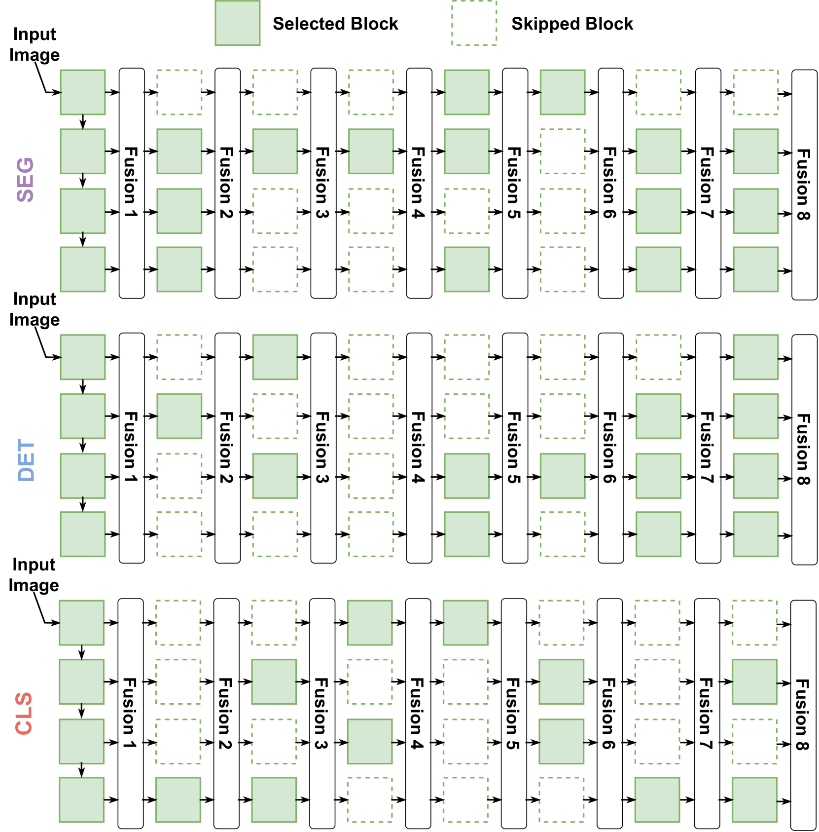
Figure 3: Visualization of the searched architectures for semantic segmentation (SEG), object detection (DET), and image classification (CLS) tasks.

5 Conclusion

We propose FBNetV5, a NAS framework that can search for neural architectures for a variety of CV tasks with reduced human effort and compute cost. FBNetV5 features a simple yet inclusive and transferable search space, a multi-task search process disentangled with target tasks’ training pipelines, and a novel search algorithm with a constant compute cost agnostic to number of tasks. Our experiments show that in a single run of search, FBNetV5 produces efficient models that significantly outperform the previous SotA models in ImageNet classification, COCO object detection, and ADE20K semantic segmentation.

6 Discussion on Limitations

There are several limitations of our work. First, we did not explore a more granular search space, e.g., to search for block-wise channel sizes, which can further improve searched models’ performance. Second, while our framework can search for multiple tasks in one run, we do not support adding new tasks incrementally, which will further improve the task-scalability. One potential solution is to explore whether we can transfer the searched architectures from one task (e.g., segmentation) to similar tasks (e.g., depth estimation) without re-running the search.

References

[1] Irwan Bello, Barret Zoph, Ashish Vaswani, Jonathon Shlens, and Quoc V Le. Attention augmented convolutional networks. In Proceedings of the IEEE/CVF International Conference on Computer Vision, pages 3286–3295, 2019.
[2] Yoshua Bengio, Nicholas Léonard, and Aaron Courville. Estimating or propagating gradients through stochastic neurons for conditional computation. arXiv preprint arXiv:1308.3432, 2013.
[3] Han Cai, Chuang Gan, Tianzhe Wang, Zhekai Zhang, and Song Han. Once-for-all: Train one network and specialize it for efficient deployment. arXiv preprint arXiv:1908.09791, 2019.
[4] Han Cai, Ligeng Zhu, and Song Han. ProxylessNAS: Direct neural architecture search on target task and hardware. arXiv preprint arXiv:1812.00332, 2018.
[5] Nicolas Carion, Francisco Massa, Gabriel Synnaeve, Nicolas Usunier, Alexander Kirillov, and Sergey Zagoruyko. End-to-end object detection with transformers. In European Conference on Computer Vision, pages 213–229. Springer, 2020.
[6] Francesco Paolo Casale, Jonathan Gordon, and Nicolo Fusi. Probabilistic neural architecture search. arXiv preprint arXiv:1902.05116, 2019.
[7] Wuyang Chen, Xinyu Gong, Xianming Liu, Qian Zhang, Yuan Li, and Zhangyang Wang. Fasterseg: Searching for faster real-time semantic segmentation. arXiv preprint arXiv:1912.10917, 2019.
[8] Xin Chen, Lingxi Xie, Jun Wu, and Qi Tian. Progressive darts: Bridging the optimization gap for NAS in the wild. arXiv preprint arXiv:1912.10952, 2019.
[9] Yukang Chen, Tong Yang, Xiangyu Zhang, Gaofeng Meng, Xinyu Xiao, and Jian Sun. DetNAS: Backbone search for object detection. Advances in Neural Information Processing Systems, 32:6642–6652, 2019.
[10] Bowen Cheng, Alexander G. Schwing, and Alexander Kirillov. Per-pixel classification is not all you need for semantic segmentation. arXiv preprint arXiv:2107.06278, 2021.
[11] Hsin-Pai Cheng, Feng Liang, Meng Li, Bowen Cheng, Feng Yan, Hai Li, Vikas Chandra, and Yiran Chen. ScaleNAS: One-shot learning of scale-aware representations for visual recognition. arXiv preprint arXiv:2011.14584, 2020.
[12] Yuanzheng Ci, Chen Lin, Ming Sun, Boyu Chen, Hongwen Zhang, and Wanli Ouyang. Evolving search space for neural architecture search. In Proceedings of the IEEE/CVF International Conference on Computer Vision (ICCV), pages 6659–6669, October 2021.
[13] Xiaoliang Dai, Alvin Wan, P. Zhang, B. Wu, Zijian He, Zhen Wei, K. Chen, Yuandong Tian, Matthew E. Yu, Péter Vajda, and J. Gonzalez. FBNetV3: Joint architecture-recipe search using neural acquisition function. ArXiv, abs/2006.02049, 2020.
[14] Xiaoliang Dai, Peizhao Zhang, Bichen Wu, Hongxu Yin, Fei Sun, Yanghan Wang, Marat Dukhan, Yunqing Hu, Yiming Wu, Yangqing Jia, et al. Chamnet: Towards efficient network design through platform-aware model adaptation. In Proceedings of the IEEE/CVF Conference on Computer Vision and Pattern Recognition, pages 11398–11407, 2019.
[15] Jia Deng, Wei Dong, Richard Socher, Li-Jia Li, Kai Li, and Li Fei-Fei. Imagenet: A large-scale hierarchical image database. In 2009 IEEE Conference on Computer Vision and Pattern Recognition, pages 248–255, 2009.
[16] Mingyu Ding, Xiaochen Lian, Linjie Yang, Peng Wang, Xiaojie Jin, Zhiwu Lu, and Ping Luo. HR-NAS: Searching efficient high-resolution neural architectures with lightweight transformers. In Proceedings of the IEEE/CVF Conference on Computer Vision and Pattern Recognition, pages 2982–2992, 2021.
[17] Xuanyi Dong and Yi Yang. NAS-bench-201: Extending the scope of reproducible neural architecture search. arXiv preprint arXiv:2001.00326, 2020.
[18] Xianzhi Du, Tsung-Yi Lin, Pengchong Jin, Golnaz Ghiasi, Mingxing Tan, Yin Cui, Quoc V Le, and Xiaodan Song. Spinenet: Learning scale-permuted backbone for recognition and localization. In Proceedings of the IEEE/CVF conference on computer vision and pattern recognition, pages 11592–11601, 2020.
[19] Zheng Ge, Songtao Liu, Feng Wang, Zeming Li, and Jian Sun. YOLOX: Exceeding YOLO series in 2021. arXiv preprint arXiv:2107.08430, 2021.
[20] Golnaz Ghiasi, Tsung-Yi Lin, and Quoc V Le. NAS-FPN: Learning scalable feature pyramid architecture for object detection. In Proceedings of the IEEE/CVF Conference on Computer Vision and Pattern Recognition, pages 7036–7045, 2019.
[21] Golnaz Ghiasi, Barret Zoph, Ekin D Cubuk, Quoc V Le, and Tsung-Yi Lin. Multi-task self-training for learning general representations. In Proceedings of the IEEE/CVF International Conference on Computer Vision, pages 8856–8865, 2021.
[22] Ben Graham, Alaaeldin El-Nouby, Hugo Touvron, Pierre Stock, Armand Joulin, Hervé Jégou, and Matthijs Douze. Levit: a vision transformer in convnet’s clothing for faster inference. arXiv preprint arXiv:2104.01136, 2021.
[23] Kaiming He, Xiangyu Zhang, Shaoqing Ren, and Jian Sun. Deep residual learning for image recognition. In Proceedings of the IEEE conference on computer vision and pattern recognition, pages 770–778, 2016.
[24] Andrew Howard, Mark Sandler, Grace Chu, Liang-Chieh Chen, Bo Chen, Mingxing Tan, Weijun Wang, Yukun Zhu, Ruoming Pang, Vijay Vasudevan, et al. Searching for MobileNetV3. In Proceedings of the IEEE/CVF International Conference on Computer Vision, pages 1314–1324, 2019.
[25] Jie Hu, Li Shen, and Gang Sun. Squeeze-and-excitation networks. In Proceedings of the IEEE conference on computer vision and pattern recognition, pages 7132–7141, 2018.
[26] Eric Jang, Shixiang Gu, and Ben Poole. Categorical reparameterization with gumbel-softmax. arXiv preprint arXiv:1611.01144, 2016.
[27] Alexander Kirillov, Ross Girshick, Kaiming He, and Piotr Dollár. Panoptic feature pyramid networks. In Proceedings of the IEEE/CVF Conference on Computer Vision and Pattern Recognition, pages 6399–6408, 2019.
[28] Changlin Li, Tao Tang, Guangrun Wang, Jiefeng Peng, Bing Wang, Xiaodan Liang, and Xiaojun Chang. BossNAS: Exploring hybrid cnn-transformers with block-wisely self-supervised neural architecture search. arXiv preprint arXiv:2103.12424, 2021.
[29] Sheng Li, Mingxing Tan, Ruoming Pang, Andrew Li, Liqun Cheng, Quoc V Le, and Norman P Jouppi. Searching for fast model families on datacenter accelerators. In Proceedings of the IEEE/CVF Conference on Computer Vision and Pattern Recognition, pages 8085–8095, 2021.
[30] Tsung-Yi Lin, Piotr Dollár, Ross Girshick, Kaiming He, Bharath Hariharan, and Serge Belongie. Feature pyramid networks for object detection. In Proceedings of the IEEE conference on computer vision and pattern recognition, pages 2117–2125, 2017.
[31] Tsung-Yi Lin, Priya Goyal, Ross Girshick, Kaiming He, and Piotr Dollár. Focal loss for dense object detection. In Proceedings of the IEEE international conference on computer vision, pages 2980–2988, 2017.
[32] Tsung-Yi Lin, Michael Maire, Serge Belongie, James Hays, Pietro Perona, Deva Ramanan, Piotr Dollár, and C Lawrence Zitnick. Microsoft coco: Common objects in context. In European conference on computer vision, pages 740–755. Springer, 2014.
[33] Hanxiao Liu, Karen Simonyan, and Yiming Yang. Darts: Differentiable architecture search. arXiv preprint arXiv:1806.09055, 2018.
[34] Shu Liu, Lu Qi, Haifang Qin, Jianping Shi, and Jiaya Jia. Path aggregation network for instance segmentation. In Proceedings of the IEEE conference on computer vision and pattern recognition, pages 8759–8768, 2018.
[35] Ze Liu, Yutong Lin, Yue Cao, Han Hu, Yixuan Wei, Zheng Zhang, Stephen Lin, and Baining Guo. Swin transformer: Hierarchical vision transformer using shifted windows. arXiv preprint arXiv:2103.14030, 2021.
[36] Ningning Ma, Xiangyu Zhang, Hai-Tao Zheng, and Jian Sun. ShuffleNet V2: Practical guidelines for efficient cnn architecture design. In Proceedings of the European conference on computer vision (ECCV), pages 116–131, 2018.
[37] Chris J Maddison, Andriy Mnih, and Yee Whye Teh. The concrete distribution: A continuous relaxation of discrete random variables. arXiv preprint arXiv:1611.00712, 2016.
[38] Art B. Owen. Monte Carlo theory, methods and examples. 2013.
[39] Adam Paszke, Sam Gross, Francisco Massa, Adam Lerer, James Bradbury, Gregory Chanan, Trevor Killeen, Zeming Lin, Natalia Gimelshein, Luca Antiga, et al. Pytorch: An imperative style, high-performance deep learning library. In Advances in neural information processing systems, pages 8026–8037, 2019.
[40] Ilija Radosavovic, Raj Prateek Kosaraju, Ross Girshick, Kaiming He, and Piotr Dollár. Designing network design spaces. In Proceedings of the IEEE/CVF Conference on Computer Vision and Pattern Recognition, pages 10428–10436, 2020.
[41] RangiLyu. Nanodet. https://github.com/RangiLyu/nanodet, 2021.
[42] Esteban Real, Sherry Moore, Andrew Selle, Saurabh Saxena, Yutaka Leon Suematsu, Jie Tan, Quoc V Le, and Alexey Kurakin. Large-scale evolution of image classifiers. In International Conference on Machine Learning, pages 2902–2911. PMLR, 2017.
[43] Shaoqing Ren, Kaiming He, Ross Girshick, and Jian Sun. Faster r-cnn: Towards real-time object detection with region proposal networks. Advances in neural information processing systems, 28:91–99, 2015.
[44] Olaf Ronneberger, Philipp Fischer, and Thomas Brox. U-net: Convolutional networks for biomedical image segmentation. In International Conference on Medical image computing and computer-assisted intervention, pages 234–241. Springer, 2015.
[45] Mark Sandler, Andrew Howard, Menglong Zhu, Andrey Zhmoginov, and Liang-Chieh Chen. Mobilenetv2: Inverted residuals and linear bottlenecks. In Proceedings of the IEEE conference on computer vision and pattern recognition, pages 4510–4520, 2018.
[46] Albert Shaw, Daniel Hunter, Forrest Landola, and Sammy Sidhu. SqueezeNAS: Fast neural architecture search for faster semantic segmentation. In Proceedings of the IEEE/CVF International Conference on Computer Vision Workshops, pages 0–0, 2019.
[47] Mingxing Tan, Bo Chen, Ruoming Pang, Vijay Vasudevan, Mark Sandler, Andrew Howard, and Quoc V Le. MnasNet: Platform-aware neural architecture search for mobile. In Proceedings of the IEEE/CVF Conference on Computer Vision and Pattern Recognition, pages 2820–2828, 2019.
[48] Mingxing Tan, Bo Chen, Ruoming Pang, Vijay Vasudevan, Mark Sandler, Andrew Howard, and Quoc V. Le. MnasNet: Platform-aware neural architecture search for mobile. In Proceedings of the IEEE/CVF Conference on Computer Vision and Pattern Recognition (CVPR), June 2019.
[49] Mingxing Tan and Quoc Le. Efficientnet: Rethinking model scaling for convolutional neural networks. In International Conference on Machine Learning, pages 6105–6114. PMLR, 2019.
[50] Mingxing Tan, Ruoming Pang, and Quoc V Le. Efficientdet: Scalable and efficient object detection. In Proceedings of the IEEE/CVF conference on computer vision and pattern recognition, pages 10781–10790, 2020.
[51] Hugo Touvron, Matthieu Cord, Matthijs Douze, Francisco Massa, Alexandre Sablayrolles, and Hervé Jégou. Training data-efficient image transformers & distillation through attention. arXiv preprint arXiv:2012.12877, 2020.
[52] Alvin Wan, Xiaoliang Dai, Peizhao Zhang, Zijian He, Yuandong Tian, Saining Xie, Bichen Wu, Matthew Yu, Tao Xu, Kan Chen, et al. FBNetV2: Differentiable neural architecture search for spatial and channel dimensions. In Proceedings of the IEEE/CVF Conference on Computer Vision and Pattern Recognition, pages 12965–12974, 2020.
[53] Dilin Wang, Chengyue Gong, Meng Li, Qiang Liu, and Vikas Chandra. AlphaNet: Improved training of supernet with alpha-divergence. arXiv preprint arXiv:2102.07954, 2021.
[54] Jingdong Wang, Ke Sun, Tianheng Cheng, Borui Jiang, Chaorui Deng, Yang Zhao, Dong Liu, Yadong Mu, Mingkui Tan, Xinggang Wang, et al. Deep high-resolution representation learning for visual recognition. IEEE transactions on pattern analysis and machine intelligence, 2020.
[55] Wenhai Wang, Enze Xie, Xiang Li, Deng-Ping Fan, Kaitao Song, Ding Liang, Tong Lu, Ping Luo, and Ling Shao. Pyramid vision transformer: A versatile backbone for dense prediction without convolutions. In IEEE ICCV, 2021.
[56] Ronald J Williams. Simple statistical gradient-following algorithms for connectionist reinforcement learning. Machine learning, 8(3):229–256, 1992.
[57] Bichen Wu, Xiaoliang Dai, Peizhao Zhang, Yanghan Wang, Fei Sun, Yiming Wu, Yuandong Tian, Peter Vajda, Yangqing Jia, and Kurt Keutzer. FBNet: Hardware-aware efficient convnet design via differentiable neural architecture search. In Proceedings of the IEEE/CVF Conference on Computer Vision and Pattern Recognition, pages 10734–10742, 2019.
[58] Yuxin Wu, Alexander Kirillov, Francisco Massa, Wan-Yen Lo, and Ross Girshick. Detectron2. https://github.com/facebookresearch/detectron2, 2019.
[59] Tete Xiao, Yingcheng Liu, Bolei Zhou, Yuning Jiang, and Jian Sun. Unified perceptual parsing for scene understanding. In Proceedings of the European Conference on Computer Vision (ECCV), pages 418–434, 2018.
[60] Enze Xie, Wenhai Wang, Zhiding Yu, Anima Anandkumar, Jose M Alvarez, and Ping Luo. Segformer: Simple and efficient design for semantic segmentation with transformers. arXiv preprint arXiv:2105.15203, 2021.
[61] Yunyang Xiong, Hanxiao Liu, Suyog Gupta, Berkin Akin, Gabriel Bender, Pieter-Jan Kindermans, Mingxing Tan, Vikas Singh, and Bo Chen. MobileDets: Searching for object detection architectures for mobile accelerators. arXiv preprint arXiv:2004.14525, 2020.
[62] Zhicheng Yan, Xiaoliang Dai, Peizhao Zhang, Yuandong Tian, Bichen Wu, and Matt Feiszli. FP-NAS: Fast probabilistic neural architecture search. In Proceedings of the IEEE/CVF Conference on Computer Vision and Pattern Recognition, pages 15139–15148, 2021.
[63] Jiahui Yu, Pengchong Jin, Hanxiao Liu, Gabriel Bender, Pieter-Jan Kindermans, Mingxing Tan, Thomas Huang, Xiaodan Song, Ruoming Pang, and Quoc Le. BigNAS: Scaling up neural architecture search with big single-stage models. In European Conference on Computer Vision, pages 702–717. Springer, 2020.
[64] Xiong Zhang, Hongmin Xu, Hong Mo, Jianchao Tan, Cheng Yang, Lei Wang, and Wenqi Ren. DCNAS: Densely connected neural architecture search for semantic image segmentation. In Proceedings of the IEEE/CVF Conference on Computer Vision and Pattern Recognition, pages 13956–13967, 2021.
[65] Bolei Zhou, Hang Zhao, Xavier Puig, Sanja Fidler, Adela Barriuso, and Antonio Torralba. Scene parsing through ade20k dataset. In Proceedings of the IEEE conference on computer vision and pattern recognition, pages 633–641, 2017.
[66] Xingyi Zhou, Vladlen Koltun, and Philipp Krähenbühl. Probabilistic two-stage detection. In arXiv preprint arXiv:2103.07461, 2021.
[67] Barret Zoph and Quoc V Le. Neural architecture search with reinforcement learning. arXiv preprint arXiv:1611.01578, 2016.

Appendix A Block Configurations of FBNetV3-A Supernet

To explain how to extend an FBNetV3[13] to the supernet in FBNetV5, we list the code snippets below. It includes the block configurations of both FBNetV3-A and the supernet extended from FBNetV3-A. It is compatible with with official implementation of FBNetV3 2 2 2 https://github.com/facebookresearch/mobile-vision/blob/main/mobile_cv/arch/fbnet_v2/fbnet_modeldef_cls_fbnetv3.py.

5[["conv_k3_hs",16,2,1]],

6[["ir_k3_hs",16,1,2,{"expansion":1}]],

8["ir_k5_hs",24,2,1,{"expansion":4}],

9["ir_k5_hs",24,1,3,{"expansion":2}],

10],

12[

13["ir_k5_sehsig_hs",40,2,1,{"expansion":5}],

14["ir_k5_sehsig_hs",40,1,4,{"expansion":3}],

15],

17[

18["ir_k5_hs",72,2,1,{"expansion":5}],

19["ir_k3_hs",72,1,4,{"expansion":3}],

20["ir_k3_sehsig_hs",120,1,1,{"expansion":5}],

21["ir_k5_sehsig_hs",120,1,5,{"expansion":3}],

22],

24[

25["ir_k3_sehsig_hs",184,2,1,{"expansion":6}],

26["ir_k5_sehsig_hs",184,1,5,{"expansion":4}],

27["ir_k5_sehsig_hs",224,1,1,{"expansion":6}],

28],

Listing 1: Code snippets of FBNetV3-A

5[["conv_k3_hs",16,2,1]],

6[["ir_k3_hs",16,1,2,{"expansion":1}]],

8["ir_k5_hs",24,2,1,{"expansion":4}],

9["ir_k5_hs",24,1,3,{"expansion":2}],

10],

12[

13["ir_k5_sehsig_hs",40,2,1,{"expansion":5}],

14["ir_k5_sehsig_hs",40,1,4,{"expansion":3}],

15],

17[

18["ir_k5_hs",72,2,1,{"expansion":5}],

19["ir_k3_hs",72,1,4,{"expansion":3}],

20["ir_k3_sehsig_hs",120,1,1,{"expansion":5}],

21["ir_k5_sehsig_hs",120,1,5,{"expansion":3}],

22],

24[

25["ir_k3_sehsig_hs",184,2,1,{"expansion":6}],

26["ir_k5_sehsig_hs",184,1,5,{"expansion":4}],

27["ir_k5_sehsig_hs",224,1,1,{"expansion":6}],

28],

30[["ir_k5_hs",24,1,2,{"expansion":2}]],

32[["ir_k5_sehsig_hs",40,1,2,{"expansion":3}]],

34[["ir_k5_sehsig_hs",120,1,2,{"expansion":3}]],

36[

37["ir_k5_sehsig_hs",224,1,1,{"expansion":4}],

38["ir_k5_sehsig_hs",224,1,1,{"expansion":6}],

39],

41[["fusion",[24,40,120,224],1,1]],

Listing 2: Code snippets of the supernet extended from FBNetV3-A

Appendix B Details about the Fusion Module

Following HRNet[54], in the supernet and searched network, we design the Fusion module to fuse feature maps with different resolutions with each other. The original HRNet’s fusion modules are computationally expensive. To reduce cost, we design a parameter-free and (almost) compute-free fusion module.

Each block in the network is fused to all blocks at the next stage. For a block at a given path: 1) if the output feature is at the same path (resolution), the fusion module is essentially a identity connection (blue arrows in Figure 4). 2) To fuse the feature to a path with larger channel size and lower resolution, we first down-sample the input feature to the target size, and repeat the original channels by ⌈C o⁢u⁢t/C i⁢n⌉subscript 𝐶 𝑜 𝑢 𝑡 subscript 𝐶 𝑖 𝑛\left\lceil C_{out}/C_{in}\right\rceil⌈ italic_C start_POSTSUBSCRIPT italic_o italic_u italic_t end_POSTSUBSCRIPT / italic_C start_POSTSUBSCRIPT italic_i italic_n end_POSTSUBSCRIPT ⌉ times, where C i⁢n,C o⁢u⁢t subscript 𝐶 𝑖 𝑛 subscript 𝐶 𝑜 𝑢 𝑡 C_{in},C_{out}italic_C start_POSTSUBSCRIPT italic_i italic_n end_POSTSUBSCRIPT , italic_C start_POSTSUBSCRIPT italic_o italic_u italic_t end_POSTSUBSCRIPT are input/output channel sizes. If C o⁢u⁢t subscript 𝐶 𝑜 𝑢 𝑡 C_{out}italic_C start_POSTSUBSCRIPT italic_o italic_u italic_t end_POSTSUBSCRIPT is not divisible by C i⁢n subscript 𝐶 𝑖 𝑛 C_{in}italic_C start_POSTSUBSCRIPT italic_i italic_n end_POSTSUBSCRIPT, we drop the extra channels. This is shown as the red arrows in Figure 4. 3) To fuse to a feature with higher resolution and smaller channel sizes, we first up-sample the feature map. Then, we pad the input feature’s channels with zero such that the channel size becomes C i⁢n′=⌈C i⁢n/C o⁢u⁢t⌉×C o⁢u⁢t subscript superscript 𝐶′𝑖 𝑛 subscript 𝐶 𝑖 𝑛 subscript 𝐶 𝑜 𝑢 𝑡 subscript 𝐶 𝑜 𝑢 𝑡 C^{\prime}{in}=\left\lceil C{in}/C_{out}\right\rceil\times C_{out}italic_C start_POSTSUPERSCRIPT ′ end_POSTSUPERSCRIPT start_POSTSUBSCRIPT italic_i italic_n end_POSTSUBSCRIPT = ⌈ italic_C start_POSTSUBSCRIPT italic_i italic_n end_POSTSUBSCRIPT / italic_C start_POSTSUBSCRIPT italic_o italic_u italic_t end_POSTSUBSCRIPT ⌉ × italic_C start_POSTSUBSCRIPT italic_o italic_u italic_t end_POSTSUBSCRIPT. Finally, we take every C i⁢n′/C o⁢u⁢t subscript superscript 𝐶′𝑖 𝑛 subscript 𝐶 𝑜 𝑢 𝑡 C^{\prime}{in}/C{out}italic_C start_POSTSUPERSCRIPT ′ end_POSTSUPERSCRIPT start_POSTSUBSCRIPT italic_i italic_n end_POSTSUBSCRIPT / italic_C start_POSTSUBSCRIPT italic_o italic_u italic_t end_POSTSUBSCRIPT channels as a group and compute a channel-wise average to produce a new output channel. This is shown as Figure 4 blue arrows. Features fused to the same block will be summed together as input to the block.

This fusion module does not require any parameters, and only requires a negligible amount of compute for down-sampling, up-sampling, padding, and channel-wise average.

In the supernet and the searched architectures, if any block (e.g., the ones in (Stage s-1, Path p) or (Stage s, Path p-1)) is skipped, the corresponding connections in the fusion modules from and to the block will also be removed, except the connections from and to other blocks in the same path.

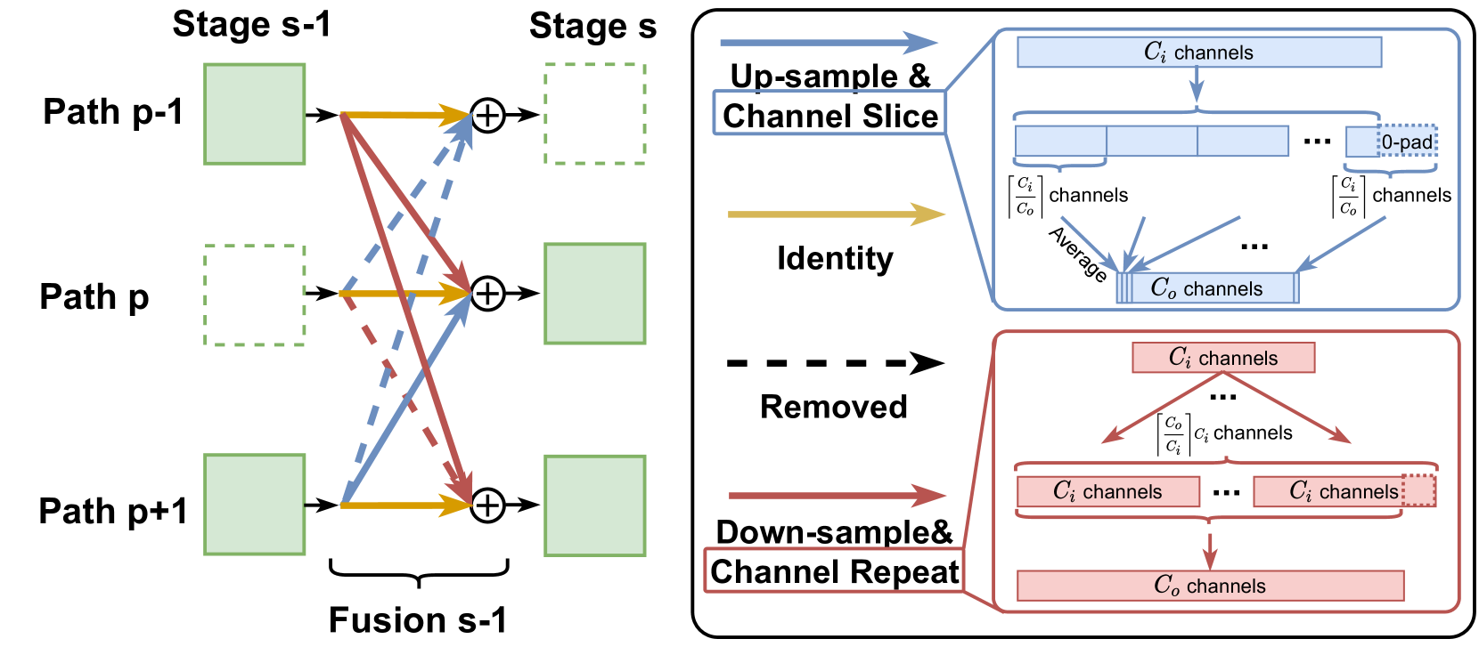
Figure 4: Illustration of the fusion module aggregating information from different paths (resolutions).

Appendix C Visualization of the Mainstream Topologies for CV Tasks

To demonstrate our search space is inclusive, we visualize how can it represent some of the mainstream network topologies for CV tasks in Figure5. These include 1) the U-Net (Figure5-top) and PANet (Figure5-middle) topology for semantic segmentation and 2) the FPN (Figure5-top) and BiFPN (Figure5-bottom) topology for object detection.

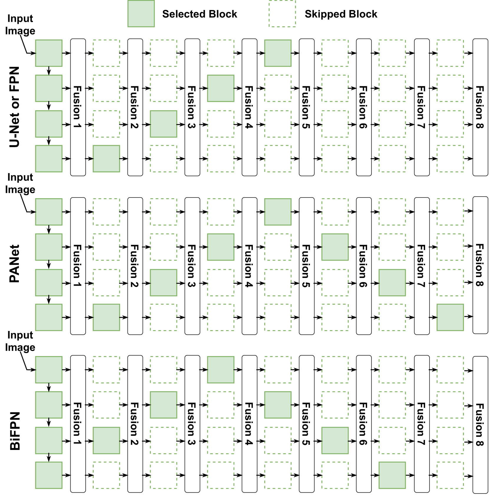
Figure 5: The search space can represent the topology of U-Net[44], PANet[34], FPN[30], and BiFPN (without the extra edge)[50].

Appendix D FBNetV3-A C and FBNetV3-A R

We provide the code snippets below to demonstrate the details about the architectures of FBNetV3-A C and FBNetV3-A R, by mainly shrinking the resolution and channel sizes from FBNetV3-A, respectively.

5[["conv_k3_hs",12,2,1]],

6[["ir_k3_hs",12,1,2,{"expansion":1}]],

8["ir_k3_hs",18,2,1,{"expansion":3}],

9["ir_k3_hs",18,1,2,{"expansion":2}],

10],

12[

13["ir_k3_sehsig_hs",30,2,1,{"expansion":4}],

14["ir_k3_sehsig_hs",30,1,3,{"expansion":2}],

15],

17[

18["ir_k3_hs",54,2,1,{"expansion":4}],

19["ir_k3_hs",54,1,3,{"expansion":2}],

20["ir_k3_sehsig_hs",80,1,1,{"expansion":4}],

21["ir_k3_sehsig_hs",80,1,3,{"expansion":2}],

22],

24[

25["ir_k3_sehsig_hs",138,2,1,{"expansion":4}],

26["ir_k3_sehsig_hs",138,1,3,{"expansion":3}],

27["ir_k3_sehsig_hs",168,1,1,{"expansion":4}],

28],

Listing 3: Code snippets of FBNetV3-A C

5[["conv_k3_hs",12,2,1]],

6[["ir_k3_hs",12,1,2,{"expansion":1}]],

8["ir_k3_hs",18,2,1,{"expansion":4}],

9["ir_k3_hs",18,1,3,{"expansion":2}],

10],

12[

13["ir_k3_sehsig_hs",30,2,1,{"expansion":5}],

14["ir_k3_sehsig_hs",30,1,4,{"expansion":3}],

15],

17[

18["ir_k3_hs",54,2,1,{"expansion":5}],

19["ir_k3_hs",54,1,4,{"expansion":3}],

20["ir_k3_sehsig_hs",80,1,1,{"expansion":5}],

21["ir_k3_sehsig_hs",80,1,5,{"expansion":3}],

22],

24[

25["ir_k3_sehsig_hs",138,2,1,{"expansion":6}],

26["ir_k3_sehsig_hs",138,1,5,{"expansion":4}],

27["ir_k3_sehsig_hs",168,1,1,{"expansion":6}],

28],

Listing 4: Code snippets of FBNetV3-A R

Appendix E Important Implementation Details of Algorithm 4

We provide several impotant implementation details of Algorithm 4.

Sampling multiple architectures. Algorithm 1 2, 3, 4 show we sample 1 architecture in each forward pass. Although it still gives an unbiased estimation of the task loss, small sample sizes lead to large variations. In practice, we implement the supernet training with distributed data parallel in Pytorch, such that each thread independently samples an architecture from the same distribution. We use 16 threads for supernet training, therefore, sampling 16 architectures per iteration to reduce the estimation variance.

Self-normalized importance sampling. In Equation (8), we compute the importance weight as r⁢(𝐚)=p 𝝅⁢(𝐚)/q⁢(𝐚)𝑟 𝐚 subscript 𝑝 𝝅 𝐚 𝑞 𝐚 r(\mathbf{a})=p_{{\bm{\pi}}}(\mathbf{a})/q(\mathbf{a})italic_r ( bold_a ) = italic_p start_POSTSUBSCRIPT bold_italic_π end_POSTSUBSCRIPT ( bold_a ) / italic_q ( bold_a ). In some extreme cases if q⁢(𝐚)𝑞 𝐚 q(\mathbf{a})italic_q ( bold_a ) is too small relative to p 𝝅⁢(𝐚)subscript 𝑝 𝝅 𝐚 p_{{\bm{\pi}}}(\mathbf{a})italic_p start_POSTSUBSCRIPT bold_italic_π end_POSTSUBSCRIPT ( bold_a ), r⁢(𝐚)𝑟 𝐚 r(\mathbf{a})italic_r ( bold_a ) will become very large that destabilize the supernet training. To prevent this, we actually use the self-normalized importance sampling and re-write Equation (8) as

𝔼 𝐚 t∼p 𝝅 t⁢{ℓ t⁢(𝐚 t,𝐰)}≈∑i=1 N r⁢(𝐚 i)⁢ℓ t⁢(𝐚 i,𝐰)∑i=1 N r⁢(𝐚 i),subscript 𝔼 similar-to superscript 𝐚 𝑡 subscript 𝑝 superscript 𝝅 𝑡 superscript ℓ 𝑡 superscript 𝐚 𝑡 𝐰 superscript subscript 𝑖 1 𝑁 𝑟 subscript 𝐚 𝑖 superscript ℓ 𝑡 subscript 𝐚 𝑖 𝐰 superscript subscript 𝑖 1 𝑁 𝑟 subscript 𝐚 𝑖\mathbb{E}{\mathbf{a}^{t}\sim p{{\bm{\pi}}^{t}}}{\ell^{t}(\mathbf{a}^{t},% \mathbf{w})}\approx\frac{\sum_{i=1}^{N}r(\mathbf{a}{i})\ell^{t}(\mathbf{a}{% i},\mathbf{w})}{\sum_{i=1}^{N}r(\mathbf{a}_{i})},blackboard_E start_POSTSUBSCRIPT bold_a start_POSTSUPERSCRIPT italic_t end_POSTSUPERSCRIPT ∼ italic_p start_POSTSUBSCRIPT bold_italic_π start_POSTSUPERSCRIPT italic_t end_POSTSUPERSCRIPT end_POSTSUBSCRIPT end_POSTSUBSCRIPT { roman_ℓ start_POSTSUPERSCRIPT italic_t end_POSTSUPERSCRIPT ( bold_a start_POSTSUPERSCRIPT italic_t end_POSTSUPERSCRIPT , bold_w ) } ≈ divide start_ARG ∑ start_POSTSUBSCRIPT italic_i = 1 end_POSTSUBSCRIPT start_POSTSUPERSCRIPT italic_N end_POSTSUPERSCRIPT italic_r ( bold_a start_POSTSUBSCRIPT italic_i end_POSTSUBSCRIPT ) roman_ℓ start_POSTSUPERSCRIPT italic_t end_POSTSUPERSCRIPT ( bold_a start_POSTSUBSCRIPT italic_i end_POSTSUBSCRIPT , bold_w ) end_ARG start_ARG ∑ start_POSTSUBSCRIPT italic_i = 1 end_POSTSUBSCRIPT start_POSTSUPERSCRIPT italic_N end_POSTSUPERSCRIPT italic_r ( bold_a start_POSTSUBSCRIPT italic_i end_POSTSUBSCRIPT ) end_ARG ,(11)

with 𝐚 i∼p 𝝅 t similar-to subscript 𝐚 𝑖 subscript 𝑝 superscript 𝝅 𝑡\mathbf{a}{i}\sim p{{\bm{\pi}}^{t}}bold_a start_POSTSUBSCRIPT italic_i end_POSTSUBSCRIPT ∼ italic_p start_POSTSUBSCRIPT bold_italic_π start_POSTSUPERSCRIPT italic_t end_POSTSUPERSCRIPT end_POSTSUBSCRIPT. This still gives an unbiased estimation [38], but will prevent the loss from becoming exceedingly large. During supernet training, we implement this through an all-gather operation to collect r⁢(𝐚 i)𝑟 subscript 𝐚 𝑖 r(\mathbf{a}_{i})italic_r ( bold_a start_POSTSUBSCRIPT italic_i end_POSTSUBSCRIPT ) from all threads and compute the normalized importance weight.

Loss normalization. In Equation (9), we scale the gradient ∇𝝅 t log⁡p 𝝅 t⁢(𝐚)subscript∇superscript 𝝅 𝑡 subscript 𝑝 superscript 𝝅 𝑡 𝐚\nabla_{{\bm{\pi}}^{t}}\log p_{{\bm{\pi}}^{t}}(\mathbf{a})∇ start_POSTSUBSCRIPT bold_italic_π start_POSTSUPERSCRIPT italic_t end_POSTSUPERSCRIPT end_POSTSUBSCRIPT roman_log italic_p start_POSTSUBSCRIPT bold_italic_π start_POSTSUPERSCRIPT italic_t end_POSTSUPERSCRIPT end_POSTSUBSCRIPT ( bold_a ) by the associated loss ℓ t⁢(𝐚)superscript ℓ 𝑡 𝐚\ell^{t}(\mathbf{a})roman_ℓ start_POSTSUPERSCRIPT italic_t end_POSTSUPERSCRIPT ( bold_a ) to determine whether we should suppress or encourage the sampled architecture 𝐚 𝐚\mathbf{a}bold_a. However, one challenge is that for different tasks, the loss ℓ t superscript ℓ 𝑡\ell^{t}roman_ℓ start_POSTSUPERSCRIPT italic_t end_POSTSUPERSCRIPT may have different mean and variance, so the gradients of different tasks can be scaled differently. To address this, instead of using the raw task-loss in Equation (9), we use a normalized task-loss, computed as ℓ^t⁢(𝐚)=(ℓ⁢(𝐚)−μ ℓ)/σ ℓ superscript^ℓ 𝑡 𝐚 ℓ 𝐚 subscript 𝜇 ℓ subscript 𝜎 ℓ\hat{\ell}^{t}(\mathbf{a})=(\ell(\mathbf{a})-\mu_{\ell})/\sigma_{\ell}over^ start_ARG roman_ℓ end_ARG start_POSTSUPERSCRIPT italic_t end_POSTSUPERSCRIPT ( bold_a ) = ( roman_ℓ ( bold_a ) - italic_μ start_POSTSUBSCRIPT roman_ℓ end_POSTSUBSCRIPT ) / italic_σ start_POSTSUBSCRIPT roman_ℓ end_POSTSUBSCRIPT, where μ ℓ,σ ℓ subscript 𝜇 ℓ subscript 𝜎 ℓ\mu_{\ell},\sigma_{\ell}italic_μ start_POSTSUBSCRIPT roman_ℓ end_POSTSUBSCRIPT , italic_σ start_POSTSUBSCRIPT roman_ℓ end_POSTSUBSCRIPT is the mean and standard deviation of the task loss in the past 200 steps. The mean μ ℓ subscript 𝜇 ℓ\mu_{\ell}italic_μ start_POSTSUBSCRIPT roman_ℓ end_POSTSUBSCRIPT provides a baseline to evaluate how does the sampled architecture 𝐚 𝐚\mathbf{a}bold_a compare with the average. This is similar to the Reinforcement Learning approach of using “advantage” instead of reward for policy gradient. The scaling factor 1/σ ℓ 1 subscript 𝜎 ℓ 1/\sigma_{\ell}1 / italic_σ start_POSTSUBSCRIPT roman_ℓ end_POSTSUBSCRIPT ensures that all losses are scaled properly without needing to tune the task-specific learning rate.

Cost regularization. In addition to the original task loss, e.g., cross-entropy for classification, we add a cost regularization term computed as λ c⁢max⁡(0,∑b a b⁢c b∑b c b−0.5)subscript 𝜆 𝑐 0 subscript 𝑏 subscript 𝑎 𝑏 subscript 𝑐 𝑏 subscript 𝑏 subscript 𝑐 𝑏 0.5\lambda_{c}\max(0,\frac{\sum_{b}a_{b}c_{b}}{\sum_{b}c_{b}}-0.5)italic_λ start_POSTSUBSCRIPT italic_c end_POSTSUBSCRIPT roman_max ( 0 , divide start_ARG ∑ start_POSTSUBSCRIPT italic_b end_POSTSUBSCRIPT italic_a start_POSTSUBSCRIPT italic_b end_POSTSUBSCRIPT italic_c start_POSTSUBSCRIPT italic_b end_POSTSUBSCRIPT end_ARG start_ARG ∑ start_POSTSUBSCRIPT italic_b end_POSTSUBSCRIPT italic_c start_POSTSUBSCRIPT italic_b end_POSTSUBSCRIPT end_ARG - 0.5 ), where c b subscript 𝑐 𝑏 c_{b}italic_c start_POSTSUBSCRIPT italic_b end_POSTSUBSCRIPT is the cost (e.g., FLOPs) of block-b 𝑏 b italic_b, and a b subscript 𝑎 𝑏 a_{b}italic_a start_POSTSUBSCRIPT italic_b end_POSTSUBSCRIPT denotes whether to select block-b or not. λ c subscript 𝜆 𝑐\lambda_{c}italic_λ start_POSTSUBSCRIPT italic_c end_POSTSUBSCRIPT is a loss coefficient. 0.5 0.5 0.5 0.5 is the relative cost target.

Warmup training. Similar to the observation of [57], before training the architecture parameters 𝝅 𝝅{\bm{\pi}}bold_italic_π, we need to first sufficiently train the model weights 𝐰 𝐰\mathbf{w}bold_w. This is because at the beginning of the supernet training, the loss will always drop regardless of the choice of architecture 𝐚 𝐚\mathbf{a}bold_a. In our implementation, we use warmup training to first train 𝐰 𝐰\mathbf{w}bold_w sufficiently and then begin to update 𝝅 𝝅{\bm{\pi}}bold_italic_π and 𝐰 𝐰\mathbf{w}bold_w jointly.

Appendix F Details about the Search and Training Process Implementation

F.1 Search Process Implementation

We introduce the implementation details of the search process of FBNetV5. As discussed in Section 3, our search is conducted by training a supernet on a multitask proxy dataset. Details of the dataset creation can be found in Section 3.2, supernet design can be found in Section 3.1. Our search is based on the supernet extended from an FBNetV3-A model as illustrated in Section3.1. On top of the supernet we use the FBNet-V3 style classification head attached to the end of Path 3. We use a Faster R-CNN head attached to Path 2 for object detection, and a single convolutional layer as the segmentation head attached to Path 2 for semantic segmentation. Note since we only care about topologies, heads used during search can be different from the heads for downstream task. We pretrain the extended supernet on the ImageNet for classification, and then train it on the multitask proxy dataset. We implement the search algorithm in D2go 3 3 3 https://github.com/facebookresearch/d2go powered by Pytorch[39] and Detectron2[58]. To train the supernet, we use a total batch size of 768. The images are resized such that the short size is 256, and we take a random crop with size 224x224 to feed to the model. We train the supernet for 9375 steps using SGD with a base learning rate of 0.96. We decay the learning rate by 10x at 3125 steps. We set the initial sampling probability of all blocks to 0.5. We do not update the architecture parameters until 6250 steps, and we the architecture parameter’s learning rate is 0.01 of the regular learning rate for weights. We use 16 V100 GPUs to train the supernet. It takes about 10 hours to finish.

F.2 Training Process Implementation

For training the task-specific architectures searched by FBNetV5, we follow existing SotA training recipes for each task[22, 10, 58] and use PyTorch[39] for all the experiments.

For ImageNet[15] image classification, we use the FBNetV3 style MBPool+FC classification head on top of the final feature map from Path 3 in Figure2. We adopt the distillation based training settings in[22, 51] and use a large pretrained model that has a 85.5% top-1 accuracy on ImageNet as the teacher model. We use a batch size of 4096 on 64 V100 GPUs for 1100 epochs, using SGD with momentum 0.9 and weight decay 2×10−5 absent superscript 10 5\times 10^{-5}× 10 start_POSTSUPERSCRIPT - 5 end_POSTSUPERSCRIPT as the optimizer, initializing the learning rate as 4.0 with 11 epochs warm-up from 0.01, and decaying it each epoch with a factor of 0.9875.

For ADE20K semantic segmentation, we modify the MaskFormer’s[10] segmentation head to a lighter version, i.e., we use a pixel decoder with a 3×\times×3 convolution layer and shrink the transformer decoder to only contain 1 Transformer layer, dubbed as Lite MaskFormer. The pixel decoder is attached to the end of Path 1, and the transformer decoder is attached to Path 3. We use the same training settings for ResNet backbone in[10] to train all the searched architectures except using 320k iterations for bigger models (FBNetV5-A/C/F-SEG in Table3) following[55]. We initialize the backbone with the weights of the ImageNet-pretrained supernet.

For COCO[32] object detection, we use the searched architectures as the backbone feature extractor. We attach a Faster R-CNN [43] head on Path 1 of the supernet. We re-design the ROI and RPN head to have a lighter architecture, and reduce the number of ROI proposals to 30 and name this version as Lite R-CNN. We follow most of the default training settings in[58] while using a batch size of 256 to train all the searched architectures for 150k iterations with a base learning rate of 0.16, and decay the learning rate by 10 after 140K steps. We keep an exponential moving average (EMA) of the model weights, and evaluate on the EMA model. The same as the settings in ADE20K above, we initialize the backbone with the weights from the ImageNet-pretrained supernet.

Appendix G Design of light Detection and Segmentation Head

G.1 Architecture of the Lite MaskFormer Head

MaskFormer[10] consists of three components, a pixel decoder (PD), a transformer decoder (TD), and a segmentation module (SM). The pixel decoder is used to generate the per-pixel embeddings. The transformer decoder is designed to output the per-segment embeddings which encode the global information of each segment. The segmentation module converts the per-segment embeddings to mask embeddings via a Multi-Layer Perceptron (MLP), and then obtain final predication via a dot product between the per-pixel embeddings from the pixel decoder and the mask embeddings.

We squeeze both the pixel decoder and the transformer decoder to build the Lite MaskFormer used in our experiments.

Our pixel decoder takes the output from Path 1 and leverage a 3×\times×3 convolution layer to generate the per-pixel embeddings.

Our transformer decoder follows the design of MaskFormer’s transformer decoder, i.e., the same with DETR[5]. But we shrink it to only contain 1 Transformer[1] layer and attach it to the output of Path 3.

We further demonstrate the distribution of our models’ FLOPs in Table6. The total FLOPs is the sum of BB, PD, TD, and SM FLOPs, and it is computed based on the input resolution of (short_size ×\times× short_size) following[10, 60].

Table 6: FLOPs of FBNetV5 segmentation models. BB, PD, TD, SM columns reports the million (M) FLOPs of the backbone, pixel decoder, transformer decoder and segmentation module of a model given the input size as (short_size ×\times× short_size). Column Total is the sum of BB, PD, TD, SM.

Model Short Size BB PD TD SM Total FBNetV5-A C-SEG 384 945 162 139 82 1328 FBNetV5-A R-SEG 384 1389 162 139 82 1773 FBNetV5-A-SEG 384 2485 215 135 84 2919 FBNetV5-C-SEG 448 3838 357 144 109 4448 FBNetV5-F-SEG 512 8502 550 155 142 9350

G.2 Architecture of the Lite Faster R-CNN Head

Table 7: FLOPs of FBNetV5 detection models. BB, RPN, ROI columns reports the million (M) FLOPs of the backbone, RPN, and ROI of a model given the reference input size. Column Total is the sum of BB, RPN, ROI. Column Avg. reports the average FLOPs of the model on the COCO val set.

Model Ref. Size BB RPN ROI Total Avg. FBNetV5-A C-DET 213x320 399 152 182 733 713 FBNetV5-A R-DET 213x320 601 152 182 935 908 FBNetV5-A-DET 213x320 1054 158 186 1398 1354 FBNetV5-A C-DET 320x481 912 347 182 1441 1367 FBNetV5-A R-DET 320x481 1372 347 182 1901 1800

For object detection, we attach Faster R-CNN[43] head to our searched backbones. Faster R-CNN detection contains two component, a region proposal network (RPN) and a region-of-interest (ROI) head. We use light-weight RPN and ROI heads to save the overall compute cost.

Our ROI head contains a inverted resitual block (IRB) [45] with kernel size 3, expansion ratio 3, output channel size 96. We also use Squeeze-Excitation [25] and HSigmoid activation following [24]. The output of RPN is fed to a single convolution layer to generate RPN output.

Our RPN head contains 4 IRB blocks with the same kernel size of 3; expansion ration of 4, 6, 6, 6; output channel size of 128, 128, 128, 160. The IRB blocks do not use SE or HSigmoid. We use an ROIPool operator to extract feature maps from a region-of-interest, and reshape the spatial size to 6x6. The first IRB block further down-samples the input resolution to 3x3. The output of the IRB blocks are projected by a single conv layer to predict ROI output (bounding box prediction, class prediction, etc.).

During inference, we select the 30 regions post NMS and feed them to ROI. Under this setting, our models FLOPs distribution is shown in Table 7. Note that the total FLOPs of our model is computed based on the reference input size. The total FLOPs is the sum of BB, RPN, and ROI FLOPs. The average FLOPs reported in Table 4 is computed based on images in the COCO val set.

Appendix H Average FLOPs of R-CNN models.

In Table 4 and Table 7, we report the average FLOPs of our model on the COCO validation dataset. This is because our R-CNN based detection model does not fix the input size, while our baselines [41, 19] takes a fixed input size. It is a more fair to use the average FLOPs of R-CNN models to compare models with a fixed input size.

During inference, our R-CNN model re-size images using the following strategy. We first define two parameters min_size (set to 224 or 320) and max_size (set to 320 or 640). For an input image, we first resize the image such that its short size becomes min_size while keeping the aspect ratio the same. After this, if the longer side the image becomes larger than max_size, we re-size the image again to make sure the longer side becomes max_size, while not changing the aspect ratio.

To compute the average FLOPs, we first compute the backbone (BB), RPN, ROI, and total flops of the model based on a reference input (e.g., 213x320 or 320x481), as in Table 7. Then, we compute the number of pixels in the reference image, and the average number of pixels for all images in the dataset. We compute a ratio ratio between the average and reference pixel number. Finally, we compute the average FLOPs as ratio x (BB + RPN) + ROI, where BB, RPN, ROI denotes the backbone, RPN, ROI FLOPs of the model. We do not scale ROI since the backbone and RPN flops is determined by the input resolution while ROI’s FLOPs do not depend on input resolution.

Xet Storage Details

Size:: 143 kB
Xet hash:: 798649fba9a387c88db701da1da2610a74f58e1074fc6ae4afb9c004a90302c7

Xet efficiently stores files, intelligently splitting them into unique chunks and accelerating uploads and downloads. More info.