2307/2307.00952.md

Title: Towards Explainable AI for Channel Estimation in Wireless Communications

URL Source: https://arxiv.org/html/2307.00952

Markdown Content: DSRC dedicated short-range communications C-ITS cooperative intelligent transport system RSU road side unit Bi bi-directional TR throughput TDL tapped delay line SRNN Simple RNN ITS Intelligent Transportation Systems IEEE Institute of Electrical and Electronics Engineers WAVE Wireless Access in Vehicular Environment V2V vehicle-to-vehicle V2I vehicle-to-infrastructure CCH control channel SCH service channels STS short training symbols LTS long training symbols SS signal symbol SoA state-of-the-art DPA data-pilot aided STA spectral temporal averaging EL ensemble learning FL frame length CDP constructed data pilots TRFI time-domain reliable test frequency domain interpolation MMSE-VP minimum mean square error using virtual pilots iCDP improved CDP SBS symbol-by-symbol FBF frame-by-frame E-TRFI Enhanced TRFI SR-CNN super resolution CNN DN-CNN denoising CNN RBF radial basis function CNN convolutional neural network TS-ChannelNet temporal spectral ChannelNet WSSUS wide-sense stationary uncorrelated scattering TDR transmission data rate LSTM long short-term memory ALS accurate LS SLS simple LS ChannelNet channel network ADD-TT average decision-directed with time truncation WI weighted interpolation DD decision-directed SR-ConvLSTM super resolution convolutional long short-term memory RS reliable subcarriers URS unreliable subcarriers AE-DNN auto-encoder deep neural network AE auto-encoder T-DFT truncated discrete Fourier transform TA-TDFT temporal averaging T-DFT TA time averaging PDP power delay profile 1G first generation 2G second generation 3G third generation 3GPP Third Generation Partnership Project 4G fourth generation 5G fifth generation 802.11 IEEE 802.11 specifications A/D analog-to-digital ADC analog-to-digital AM amplitude modulation AP access point AR augmented reality ASIC application-specific integrated circuit ASIP Application Specific Integrated Processors AWGN additive white Gaussian noise BCJR Bahl, Cocke, Jelinek and Raviv BER bit error rate BFDM bi-orthogonal frequency division multiplexing BPSK binary phase shift keying BS base stations CA carrier aggregation CAF cyclic autocorrelation function Car-2-x car-to-car and car-to-infrastructure communication CAZAC constant amplitude zero autocorrelation waveform CB-FMT cyclic block filtered multitone CCDF complementary cumulative density function CDF cumulative density function CDMA code-division multiple access CFO carrier frequency offset CIR channel impulse response CM complex multiplication COFDM coded-OFDMCoMP coordinated multi point COQAM cyclic OQAM CP cyclic prefix CR cognitive radio CRC cyclic redundancy check CRLB Cramér-Rao lower bound CS cyclic suffix CSI channel state information CSMA carrier-sense multiple access CWCU component-wise conditionally unbiased D/A digital-to-analog D2D device-to-device DAC digital-to-analog DC direct current DFE decision feedback equalizer DFT discrete Fourier transform DL deep learning DMT discrete multitone DNN deep neural network FNN feed-forward neural network DSA dynamic spectrum access DSL digital subscriber line DSP digital signal processor DTFT discrete-time Fourier transform DVB digital video broadcasting DVB-T terrestrial digital video broadcasting DWMT discrete wavelet multi tone DZT discrete Zak transform E2E end-to-end eNodeB evolved node b base station E-SNR effective signal-to-noise ratio EVD eigenvalue decomposition FBMC filter bank multicarrier FD frequency-domain FDD frequency-division duplexing FDE frequency domain equalization FDM frequency division multiplex FDMA frequency-division multiple access FEC forward error correction FER frame error rate FFT fast Fourier transform FIR finite impulse response FM frequency modulation FMT filtered multi tone FO frequency offset F-OFDM filtered-OFDMFPGA field programmable gate array FSC frequency selective channel FS-OQAM-GFDM frequency-shift OQAM-GFDM FT Fourier transform FTD fractional time delay FTN faster-than-Nyquist signaling GFDM generalized frequency division multiplexing GFDMA generalized frequency division multiple access GMC-CDM generalized multicarrier code-division multiplexing GNSS global navigation satellite system GS guard symbols GSM Groupe Spécial Mobile GUI graphical user interface H2H human-to-human H2M human-to-machine HTC human type communication I in-phase i.i.d.independent and identically distributed IB in-band IBI inter-block interference IC interference cancellation ICI inter-carrier interference ICT information and communication technologies ICV information coefficient vector IDFT inverse discrete Fourier transform IDMA interleave division multiple access IEEE institute of electrical and electronics engineers IF intermediate frequency IFFT inverse fast Fourier transform IoT Internet of Things IOTA isotropic orthogonal transform algorithm IP internet protocole IP-core intellectual property core ISDB-T terrestrial integrated services digital broadcasting ISDN integrated services digital network ISI inter-symbol interference ITU International Telecommunication Union IUI inter-user interference LAN local area netwrok LLR log-likelihood ratio LMMSE linear minimum mean square error LNA low noise amplifier LO local oscillator LOS line-of-sight LP low-pass LPF low-pass filter LS least squares LTE Long Term Evolution LTE-A LTE-Advanced LTIV linear time invariant LTV linear time-variant LUT lookup table M2M machine-to-machine MA multiple access MAC multiple access control MAP maximum a posteriori MC multicarrier MCA multicarrier access MCM multicarrier modulation MCS modulation coding scheme MF matched filter MF-SIC matched filter with successive interference cancellation MIMO multiple-input, multiple-output MISO multiple-input single-output ML machien learning MLD maximum likelihood detection MLE maximum likelihood estimator MMSE minimum mean squared error MRC maximum ratio combining MS mobile stations MSE mean squared error MSK Minimum-shift keying MSSS mean-square signal separation MTC machine type communication MU multi user MVUE minimum variance unbiased estimator NEF noise enhancement factor NLOS non-line-of-sight NMSE normalized mean-squared error NOMA non-orthogonal multiple access NPR near-perfect reconstruction NRZ non-return-to-zero OFDM orthogonal frequency division multiplexing OFDMA orthogonal frequency division multiple access OOB out-of-band OQAM offset quadrature amplitude modulation OQPSK offset quadrature phase shift keying OTFS orthogonal time frequency space PA power amplifier PAM pulse amplitude modulation PAPR peak-to-average power ratio PC-CC parallel concatenated convolutional code PCP pseudo-circular pre/post-amble PD probability of detection pdf probability density function PDF probability distribution function PFA probability of false alarm PHY physical layer PIC parallel interference cancellation PLC power line communication PMF probability mass function PN pseudo noise ppm parts per million PRB physical resource block PRB physical resource block PSD power spectral density Q quadrature-phase QAM quadrature amplitude modulation QoS quality of service QPSK quadrature phase shift keying R/W read-or-write RAM random-access memmory RAN radio access network RAT radio access technologies RC raised cosine RF radio frequency rms root mean square RRC root raised cosine RW read-and-write SC single-carrier SCA single-carrier access SC-FDE single-carrier with frequency domain equalization SC-FDM single-carrier frequency division multiplexing SC-FDMA single-carrier frequency division multiple access SD sphere decoding SDD space-division duplexing SDMA space division multiple access SDR software-defined radio SDW software-defined waveform SEFDM spectrally efficient frequency division multiplexing SE-FDM spectrally efficient frequency division multiplexing SER symbol error rate SIC successive interference cancellation SINR signal-to-interference-plus-noise ratio SIR signal-to-interference ratio SISO single-input, single-output SMS Short Message Service SNR signal-to-noise ratio STC space-time coding STFT short-time Fourier transform STO symbol time offset SU single user AI Artificial intelligence SVD singular value decomposition TD time-domain TDD time-division duplexing TDMA time-division multiple access TFL time-frequency localization TO time offset TS-OQAM-GFDM time-shifted OQAM-GFDM XAI explainable AI UE user equipment VTV-US Vehicle-to-Vehicle urban scenario VTI-US Vehicle-to-Infrastructure urban scenario UFMC universally filtered multicarrier UL uplink US uncorrelated scattering USB universal serial bus UW unique word VLC visible light communications VR virtual reality WCP windowing and CPANN artificial neural network GRU gated recurrent unit RNN recurrent neural network WHT Walsh-Hadamard transform WiMAX worldwide interoperability for microwave access WLAN wireless local area network W-OFDM windowed-OFDMWOLA windowing and overlapping WSS wide-sense stationary ZCT Zadoff-Chu transform ZF zero-forcing ZMCSCG zero-mean circularly-symmetric complex Gaussian ZP zero-padding ZT zero-tail Abdul Karim Gizzini,Yahia Medjahdi,Ali J.Ghandour,Laurent Clavier Abdul Karim Gizzini, Yahia Medjahdi, and Laurent Clavier are with the Center for Digital Systems, IMT Nord Europe, Institut Mines-Télécom, University of Lille, France (e-mail: {abdul-karim.gizzini, yahia.medjahdi,laurent.clavier}@imt-nord-europe.fr). Ali J. Ghandour is with the National Center for Remote Sensing - CNRS, Lebanon (e-mail: aghandour@cnrs.edu.lb).

Abstract

Research into 6G networks has been initiated to support a variety of critical artificial intelligence (AI) assisted applications such as autonomous driving. In such applications, AI-based decisions should be performed in a real-time manner. These decisions include resource allocation, localization, channel estimation, etc. Considering the black-box nature of existing AI-based models, it is highly challenging to understand and trust the decision-making behavior of such models. Therefore, explaining the logic behind those models through explainable AI (XAI) techniques is essential for their employment in critical applications. This manuscript proposes a novel XAI-based channel estimation (XAI-CHEST) scheme that provides detailed reasonable interpretability of the deep learning (DL) models that are employed in doubly-selective channel estimation. The aim of the proposed XAI-CHEST scheme is to identify the relevant model inputs by inducing high noise on the irrelevant ones. As a result, the behavior of the studied DL-based channel estimators can be further analyzed and evaluated based on the generated interpretations. Simulation results show that the proposed XAI-CHEST scheme provides valid interpretations of the DL-based channel estimators for different scenarios.

Index Terms:

6G, AI, XAI, channel estimation, XAI-CHEST

I Introduction

It is envisioned that 6G technology will provide a new era of mass digital connectivity and automation of several advanced smart services such as autonomous driving and remote surgery[1]. Such services are mission critical, where high data rates, low latency, and robust communications must be established and guaranteed[2]. Artificial intelligence (AI) will be a key element in future smart applications, due to its great success in providing good performance compared to conventional methods. However, the recent deep learning (DL)-based schemes proposed for wireless communications suffer mainly from the lack of transparency and trust. In this context, the development of trustworthy DL-based schemes is a crucial need in order to provide explainability for the DL model decisions in a logical and understandable manner[1, 3, 4]. Motivated by the fact that reliable communications can be guaranteed by accurate channel estimation, recently, DL algorithms have been integrated into channel estimation[5] to handle the limitations of conventional channel estimators represented by prior data knowledge, high complexity and statistical assumptions. These limitations lead to significant performance degradation, especially in doubly-selective environments, where the channel varies in both time and frequency. In contrast, DL-based channel estimators have succeeded in improving the overall system performance, especially when used on top of low-complexity conventional estimators. This success is mainly due to the robustness, low complexity, and good generalization ability of DL techniques. This generalization ability can be guaranteed by employing several techniques like the Bayesian neural network (BNN). Unlike regular DL networks where the weights are considered as point estimates, thus, they may suffer from the overfitting problem, i.e. lack of a good generalization capability for new samples in the testing phase. BNN networks are able to tackle this issue by placing the point estimates with probability distributions, where they measure the model uncertainty resulting from the input data and model training[6, 7]. After that, BNN applies the desired regularization according to measured uncertainty, where better generalization can be achieved.

Even though DL-based channel estimators provide a good generalization and performance-complexity trade-off, they lack decision-making interpretability. Hence, they are classified as black-box DL models with a main trustworthiness problem. This lack of interpretability can be addressed by developing explainable AI (XAI) schemes that increase the black-box models transparency and explain why certain decisions were made. XAI schemes are able to provide reasoning and justifications of the DL behavior, thus, transforming the black-box model into a white-box model and ensuring the adaptation, trustfulness and transparency of a given model. A variety of DL techniques are employed in the doubly-selective channel estimation[8, 9], however, this paper considers the recently proposed feed-forward neural network (FNN)-based channel estimators[10, 11].

According to the XAI taxonomy, as shown in Fig.1, there are two main categories of XAI methods[12]: (i) perturbation-based or gradient-free methods, where the concept is to perturb input features by masking or altering their values and record the effect of these changes on the model performance and (ii) gradient-based methods where the gradients of the output are calculated with respect to the input via back-propagation and used to estimate importance scores of the input features.

In this context, XAI schemes can be further classified into (i) model-Agnostic: where the XAI scheme does not consider the internal architecture of the model including the weights and the layers. Hence, Agnostic-based XAI schemes are characterized by high flexibility since they can be applied to interpret any black-box model regardless of its architecture. (ii) model-specific: Here the XAI scheme is defined according to the architecture and parameters of a specific trained model. Thus it can not be employed for a variety of DL models.

It should be noted that XAI schemes are used primarily in computer vision applications[13]. Procedures and methodology for adopting and deploying such schemes in the wireless communications discipline are still unclear[1]. In this context, this paper proposes a novel model-agnostic perturbation-based XAI channel estimation (XAI-CHEST) scheme, where the interpretability of recently proposed FNN-based channel estimators is investigated. The key idea is to employ an FNN model, denoted as the interpretability model, to provide interpretations for the considered black-box model denoted as the utility model. The interpretability model role is to induce noise on the FNN inputs without degrading the performance of the utility model. To achieve this, the interpretability model will only induce high noise on the FNN inputs that are not substantial to the utility model proper functioning. As a result, the interpretability model generates a noise mask that includes the corresponding noise weight for each FNN input, where the FNN inputs can be classified as either relevant or irrelevant inputs. Simulation results reveal that the proposed XAI-CHEST scheme is able to accurately illustrate the behavior of the utility model, thus transforming it into a white-box model. Furthermore, we show that employing only selected relevant inputs instead of the full inputs improves the FNN-based channel estimators performance.

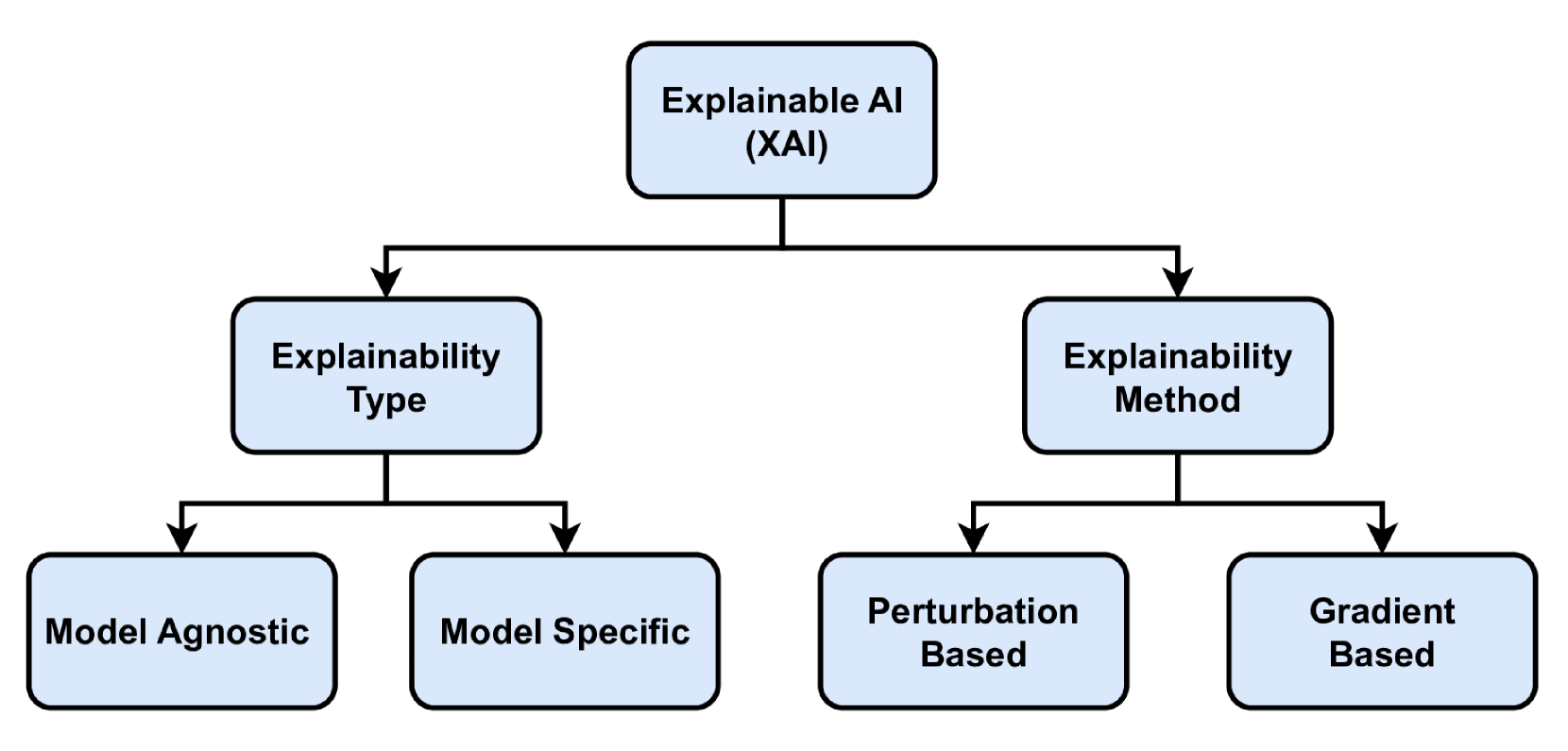
Fig. 1: General XAI taxonomy.

To the best of our knowledge, this is the first work to propose an XAI scheme for physical layer applications in wireless communications, specifically, channel estimation. In summary, the contributions of this paper are threefolds

• • Proposing an XAI-CHEST scheme that provides detailed interpretability to the recently proposed FNN-based channel estimators.

• • Showing that the interpretability of the studied FNN models can be achieved by inducing noise on the model inputs while maximizing their accuracy. Therefore, the inputs of the model are classified into relevant and irrelevant sets based on the induced noise mask.

• • Providing an extensive performance evaluation of the proposed XAI-CHEST scheme in different scenarios, where we show that using only relevant inputs instead of the full set improves the performance of the studied FNN-based channel estimators, as well as reducing the computational complexity.

The remainder of this paper is organized as follows: SectionII presents the system model. The DL-based channel estimators to be interpreted are presented in SectionIII. SectionIV illustrates the proposed XAI-CHEST scheme. In SectionV, the performance of the proposed XAI-CHEST scheme in terms of bit error rate (BER) is analyzed. Finally, SectionVI concludes the manuscript.

II System Model

Consider a frame consisting of I 𝐼 I italic_Iorthogonal frequency division multiplexing (OFDM) symbols. The i 𝑖 i italic_i-th transmitted frequency-domain OFDM subcarrier 𝒙i⁢[k]subscript𝒙 𝑖 delimited-[]𝑘\tilde{\bm{x}}_{i}[k]over~ start_ARG bold_italic_x end_ARG start_POSTSUBSCRIPT italic_i end_POSTSUBSCRIPT [ italic_k ], is denoted by

𝒙i⁢[k]={𝒙i,d⁢[k],k∈𝒦 d 𝒙i,p⁢[k],k∈𝒦 p 0,k∈𝒦 n subscript𝒙 𝑖 delimited-[]𝑘 cases subscript𝒙 𝑖 𝑑 delimited-[]𝑘 𝑘 subscript 𝒦 d subscript𝒙 𝑖 𝑝 delimited-[]𝑘 𝑘 subscript 𝒦 p 0 𝑘 subscript 𝒦 n\tilde{\bm{x}}{i}[k]=\left{\begin{array}[]{ll}\tilde{\bm{x}}{{i,d}}[k],&% \quad k\in{\mathcal{K}}{\text{d}}\ \tilde{\bm{x}}{{i,p}}[k],&\quad k\in{\mathcal{K}}{\text{p}}\ 0,&\quad k\in{\mathcal{K}}{\text{n}}\ \end{array}\right.over~ start_ARG bold_italic_x end_ARG start_POSTSUBSCRIPT italic_i end_POSTSUBSCRIPT [ italic_k ] = { start_ARRAY start_ROW start_CELL over~ start_ARG bold_italic_x end_ARG start_POSTSUBSCRIPT italic_i , italic_d end_POSTSUBSCRIPT [ italic_k ] , end_CELL start_CELL italic_k ∈ caligraphic_K start_POSTSUBSCRIPT d end_POSTSUBSCRIPT end_CELL end_ROW start_ROW start_CELL over~ start_ARG bold_italic_x end_ARG start_POSTSUBSCRIPT italic_i , italic_p end_POSTSUBSCRIPT [ italic_k ] , end_CELL start_CELL italic_k ∈ caligraphic_K start_POSTSUBSCRIPT p end_POSTSUBSCRIPT end_CELL end_ROW start_ROW start_CELL 0 , end_CELL start_CELL italic_k ∈ caligraphic_K start_POSTSUBSCRIPT n end_POSTSUBSCRIPT end_CELL end_ROW end_ARRAY(1)

where 0≤k≤K−1 0 𝑘 𝐾 1 0\leq k\leq K-1 0 ≤ italic_k ≤ italic_K - 1. The total number of used subcarriers is divided into K on=K d+K p subscript 𝐾 on subscript 𝐾 𝑑 subscript 𝐾 𝑝 K_{\text{on}}=K_{d}+K_{p}italic_K start_POSTSUBSCRIPT on end_POSTSUBSCRIPT = italic_K start_POSTSUBSCRIPT italic_d end_POSTSUBSCRIPT + italic_K start_POSTSUBSCRIPT italic_p end_POSTSUBSCRIPT subcarriers in addition to K n subscript 𝐾 𝑛 K_{n}italic_K start_POSTSUBSCRIPT italic_n end_POSTSUBSCRIPT null guard band subcarriers, where 𝒙i,d∈ℂ K d×1 subscript𝒙 𝑖 𝑑 superscript ℂ subscript 𝐾 𝑑 1\tilde{\bm{x}}{{i,d}}\in\mathbb{C}^{K{d}\times 1}over~ start_ARG bold_italic_x end_ARG start_POSTSUBSCRIPT italic_i , italic_d end_POSTSUBSCRIPT ∈ blackboard_C start_POSTSUPERSCRIPT italic_K start_POSTSUBSCRIPT italic_d end_POSTSUBSCRIPT × 1 end_POSTSUPERSCRIPT and 𝒙i,p∈ℂ K p×1 subscript𝒙 𝑖 𝑝 superscript ℂ subscript 𝐾 𝑝 1\tilde{\bm{x}}{{i,p}}\in\mathbb{C}^{K{p}\times 1}over~ start_ARG bold_italic_x end_ARG start_POSTSUBSCRIPT italic_i , italic_p end_POSTSUBSCRIPT ∈ blackboard_C start_POSTSUPERSCRIPT italic_K start_POSTSUBSCRIPT italic_p end_POSTSUBSCRIPT × 1 end_POSTSUPERSCRIPT represent the modulated data symbols and the predefined pilot symbols allocated at a set of subcarriers denoted 𝒦 d subscript 𝒦 d{\mathcal{K}}{\text{d}}caligraphic_K start_POSTSUBSCRIPT d end_POSTSUBSCRIPT and 𝒦 p subscript 𝒦 p{\mathcal{K}}{\text{p}}caligraphic_K start_POSTSUBSCRIPT p end_POSTSUBSCRIPT, respectively. The received frequency-domain OFDM subcarrier denoted as 𝒚i⁢[k]subscript𝒚 𝑖 delimited-[]𝑘\tilde{\bm{y}}_{{i}}[k]over~ start_ARG bold_italic_y end_ARG start_POSTSUBSCRIPT italic_i end_POSTSUBSCRIPT [ italic_k ] is expressed as follows:

𝒚i⁢[k]=𝒉i⁢[k]⁢𝒙i⁢[k]+𝒆i⁢[k]+𝒗i⁢[k],k∈𝒦 on formulae-sequence subscript𝒚 𝑖 delimited-[]𝑘 subscript𝒉 𝑖 delimited-[]𝑘 subscript𝒙 𝑖 delimited-[]𝑘 subscript𝒆 𝑖 delimited-[]𝑘 subscript𝒗 𝑖 delimited-[]𝑘 𝑘 subscript 𝒦 on\begin{split}\tilde{\bm{y}}{{i}}[k]&=\tilde{\bm{h}}{i}[k]\tilde{\bm{x}}{i}[% k]+\tilde{\bm{e}}{i}[k]+\tilde{\bm{v}}{i}[k],\leavevmode\nobreak\ k\in{% \mathcal{K}}{\text{on}}\end{split}start_ROW start_CELL over~ start_ARG bold_italic_y end_ARG start_POSTSUBSCRIPT italic_i end_POSTSUBSCRIPT [ italic_k ] end_CELL start_CELL = over~ start_ARG bold_italic_h end_ARG start_POSTSUBSCRIPT italic_i end_POSTSUBSCRIPT [ italic_k ] over~ start_ARG bold_italic_x end_ARG start_POSTSUBSCRIPT italic_i end_POSTSUBSCRIPT [ italic_k ] + over~ start_ARG bold_italic_e end_ARG start_POSTSUBSCRIPT italic_i end_POSTSUBSCRIPT [ italic_k ] + over~ start_ARG bold_italic_v end_ARG start_POSTSUBSCRIPT italic_i end_POSTSUBSCRIPT [ italic_k ] , italic_k ∈ caligraphic_K start_POSTSUBSCRIPT on end_POSTSUBSCRIPT end_CELL end_ROW(2)

where 𝒚i∈ℂ K o⁢n×1 subscript𝒚 𝑖 superscript ℂ subscript 𝐾 𝑜 𝑛 1\tilde{\bm{y}}{i}\in\mathbb{C}^{K{on}\times 1}over~ start_ARG bold_italic_y end_ARG start_POSTSUBSCRIPT italic_i end_POSTSUBSCRIPT ∈ blackboard_C start_POSTSUPERSCRIPT italic_K start_POSTSUBSCRIPT italic_o italic_n end_POSTSUBSCRIPT × 1 end_POSTSUPERSCRIPT and 𝒙i∈ℂ K o⁢n×1 subscript𝒙 𝑖 superscript ℂ subscript 𝐾 𝑜 𝑛 1\tilde{\bm{x}}{i}\in\mathbb{C}^{K{on}\times 1}over~ start_ARG bold_italic_x end_ARG start_POSTSUBSCRIPT italic_i end_POSTSUBSCRIPT ∈ blackboard_C start_POSTSUPERSCRIPT italic_K start_POSTSUBSCRIPT italic_o italic_n end_POSTSUBSCRIPT × 1 end_POSTSUPERSCRIPT represents the received and transmitted OFDM symbols, respectively. 𝒉i∈ℂ K o⁢n×1 subscript𝒉 𝑖 superscript ℂ subscript 𝐾 𝑜 𝑛 1\tilde{\bm{h}}{i}\in\mathbb{C}^{K{on}\times 1}over~ start_ARG bold_italic_h end_ARG start_POSTSUBSCRIPT italic_i end_POSTSUBSCRIPT ∈ blackboard_C start_POSTSUPERSCRIPT italic_K start_POSTSUBSCRIPT italic_o italic_n end_POSTSUBSCRIPT × 1 end_POSTSUPERSCRIPT refers to the frequency response of the doubly-selective channel at the i 𝑖 i italic_i-th OFDM. 𝒗i∈ℂ K o⁢n×1 subscript𝒗 𝑖 superscript ℂ subscript 𝐾 𝑜 𝑛 1{\tilde{\bm{v}}}{i}\in\mathbb{C}^{K{on}\times 1}over~ start_ARG bold_italic_v end_ARG start_POSTSUBSCRIPT italic_i end_POSTSUBSCRIPT ∈ blackboard_C start_POSTSUPERSCRIPT italic_K start_POSTSUBSCRIPT italic_o italic_n end_POSTSUBSCRIPT × 1 end_POSTSUPERSCRIPT signifies the additive white Gaussian noise (AWGN) of variance σ 2 superscript 𝜎 2\sigma^{2}italic_σ start_POSTSUPERSCRIPT 2 end_POSTSUPERSCRIPT and 𝒆i∈ℂ K o⁢n×1 subscript𝒆 𝑖 superscript ℂ subscript 𝐾 𝑜 𝑛 1\tilde{\bm{e}}{i}\in\mathbb{C}^{K{on}\times 1}over~ start_ARG bold_italic_e end_ARG start_POSTSUBSCRIPT italic_i end_POSTSUBSCRIPT ∈ blackboard_C start_POSTSUPERSCRIPT italic_K start_POSTSUBSCRIPT italic_o italic_n end_POSTSUBSCRIPT × 1 end_POSTSUPERSCRIPT denotes the Doppler interference derived in[8].

III DL-based Channel Estimation Schemes

Conventional channel estimators are based on preamble-based channel estimation, where the channel is estimated once at the beginning of the received frame. In this case, the estimated channel becomes outdated in high-mobility environments. Pilot subcarriers allocated within a transmitted OFDM symbol are limited and cannot fully capture the doubly selective channel variations. In this context, several channel estimators are proposed in the literature to allow better channel tracking over time, where FNN is applied as a post-processing on top of conventional channel estimators. In this work, the interpretability of the recently proposed spectral temporal averaging (STA)-FNN and time-domain reliable test frequency domain interpolation (TRFI)-FNN channel estimators is investigated.

III-A STA-FNN

In the STA estimator[14], frequency- and time- domain averaging are applied on top of the data-pilot aided (DPA) channel estimation. We note that DPA channel estimation utilizes the demapped data subcarriers of the previously received OFDM symbol to estimate the channel for the current OFDM symbol such that

𝒅i⁢[k]=𝔇⁢(𝒚i⁢[k]𝒉^DPA i−1⁢[k]),𝒉^DPA 0⁢[k]=𝒉^LS⁢[k]formulae-sequence subscript𝒅 𝑖 delimited-[]𝑘 𝔇 subscript𝒚 𝑖 delimited-[]𝑘 subscript^𝒉 subscript DPA 𝑖 1 delimited-[]𝑘 subscript^𝒉 subscript DPA 0 delimited-[]𝑘 subscript^𝒉 LS delimited-[]𝑘\tilde{\bm{d}}{i}[k]=\mathfrak{D}\big{(}\frac{\tilde{\bm{y}}{i}[k]}{\hat{% \tilde{\bm{h}}}{\text{DPA}{i-1}}[k]}\big{)},\leavevmode\nobreak\ \hat{\tilde% {\bm{h}}}{\text{DPA}{0}}[k]=\hat{\tilde{\bm{h}}}_{\text{LS}}[k]over~ start_ARG bold_italic_d end_ARG start_POSTSUBSCRIPT italic_i end_POSTSUBSCRIPT [ italic_k ] = fraktur_D ( divide start_ARG over~ start_ARG bold_italic_y end_ARG start_POSTSUBSCRIPT italic_i end_POSTSUBSCRIPT [ italic_k ] end_ARG start_ARG over^ start_ARG over~ start_ARG bold_italic_h end_ARG end_ARG start_POSTSUBSCRIPT DPA start_POSTSUBSCRIPT italic_i - 1 end_POSTSUBSCRIPT end_POSTSUBSCRIPT [ italic_k ] end_ARG ) , over^ start_ARG over~ start_ARG bold_italic_h end_ARG end_ARG start_POSTSUBSCRIPT DPA start_POSTSUBSCRIPT 0 end_POSTSUBSCRIPT end_POSTSUBSCRIPT [ italic_k ] = over^ start_ARG over~ start_ARG bold_italic_h end_ARG end_ARG start_POSTSUBSCRIPT LS end_POSTSUBSCRIPT italic_k

where 𝔇(.)\mathfrak{D}(.)fraktur_D ( . ) refers to the demapping operation to the nearest constellation point in accordance with the employed modulation order. 𝒉^LS subscript^𝒉 LS\hat{\tilde{\bm{h}}}_{\text{LS}}over^ start_ARG over~ start_ARG bold_italic_h end_ARG end_ARG start_POSTSUBSCRIPT LS end_POSTSUBSCRIPT stands for the LS estimated channel at the received preambles. Thereafter, the final DPA channel estimates are updated in the following manner

𝒉^DPA i⁢[k]=𝒚i⁢[k]𝒅i⁢[k]subscript^𝒉 subscript DPA 𝑖 delimited-[]𝑘 subscript𝒚 𝑖 delimited-[]𝑘 subscript𝒅 𝑖 delimited-[]𝑘\hat{\tilde{\bm{h}}}{\text{DPA}{i}}[k]=\frac{\tilde{\bm{y}}{i}[k]}{\tilde{% \bm{d}}{i}[k]}over^ start_ARG over~ start_ARG bold_italic_h end_ARG end_ARG start_POSTSUBSCRIPT DPA start_POSTSUBSCRIPT italic_i end_POSTSUBSCRIPT end_POSTSUBSCRIPT [ italic_k ] = divide start_ARG over~ start_ARG bold_italic_y end_ARG start_POSTSUBSCRIPT italic_i end_POSTSUBSCRIPT [ italic_k ] end_ARG start_ARG over~ start_ARG bold_italic_d end_ARG start_POSTSUBSCRIPT italic_i end_POSTSUBSCRIPT [ italic_k ] end_ARG(4)

Finally, frequency- and time- domain averaging are implemented as follows:

𝒉^FD i⁢[k]=∑λ=−β λ=β ω λ⁢𝒉^DPA i⁢[k+λ],ω λ=1 2⁢β+1 formulae-sequence subscript^𝒉 subscript FD 𝑖 delimited-[]𝑘 superscript subscript 𝜆 𝛽 𝜆 𝛽 subscript 𝜔 𝜆 subscript^𝒉 subscript DPA 𝑖 delimited-[]𝑘 𝜆 subscript 𝜔 𝜆 1 2 𝛽 1\hat{\tilde{\bm{h}}}{\text{FD}{i}}[k]=\sum_{\lambda=-\beta}^{\lambda=\beta}% \omega_{\lambda}\hat{\tilde{\bm{h}}}{\text{DPA}{i}}[k+\lambda],\leavevmode% \nobreak\ \omega_{\lambda}=\frac{1}{2\beta+1}over^ start_ARG over~ start_ARG bold_italic_h end_ARG end_ARG start_POSTSUBSCRIPT FD start_POSTSUBSCRIPT italic_i end_POSTSUBSCRIPT end_POSTSUBSCRIPT [ italic_k ] = ∑ start_POSTSUBSCRIPT italic_λ = - italic_β end_POSTSUBSCRIPT start_POSTSUPERSCRIPT italic_λ = italic_β end_POSTSUPERSCRIPT italic_ω start_POSTSUBSCRIPT italic_λ end_POSTSUBSCRIPT over^ start_ARG over~ start_ARG bold_italic_h end_ARG end_ARG start_POSTSUBSCRIPT DPA start_POSTSUBSCRIPT italic_i end_POSTSUBSCRIPT end_POSTSUBSCRIPT [ italic_k + italic_λ ] , italic_ω start_POSTSUBSCRIPT italic_λ end_POSTSUBSCRIPT = divide start_ARG 1 end_ARG start_ARG 2 italic_β + 1 end_ARG(5)

𝒉^STA i⁢[k]=(1−1 α)⁢𝒉^STA i−1⁢[k]+1 α⁢𝒉^FD i⁢[k]subscript^𝒉 subscript STA 𝑖 delimited-[]𝑘 1 1 𝛼 subscript^𝒉 subscript STA 𝑖 1 delimited-[]𝑘 1 𝛼 subscript^𝒉 subscript FD 𝑖 delimited-[]𝑘\hat{\tilde{\bm{h}}}{\text{STA}{i}}[k]=(1-\frac{1}{\alpha})\hat{\tilde{\bm{h% }}}{\text{STA}{i-1}}[k]+\frac{1}{\alpha}\hat{\tilde{\bm{h}}}{\text{FD}{i}}% [k]over^ start_ARG over~ start_ARG bold_italic_h end_ARG end_ARG start_POSTSUBSCRIPT STA start_POSTSUBSCRIPT italic_i end_POSTSUBSCRIPT end_POSTSUBSCRIPT [ italic_k ] = ( 1 - divide start_ARG 1 end_ARG start_ARG italic_α end_ARG ) over^ start_ARG over~ start_ARG bold_italic_h end_ARG end_ARG start_POSTSUBSCRIPT STA start_POSTSUBSCRIPT italic_i - 1 end_POSTSUBSCRIPT end_POSTSUBSCRIPT [ italic_k ] + divide start_ARG 1 end_ARG start_ARG italic_α end_ARG over^ start_ARG over~ start_ARG bold_italic_h end_ARG end_ARG start_POSTSUBSCRIPT FD start_POSTSUBSCRIPT italic_i end_POSTSUBSCRIPT end_POSTSUBSCRIPT italic_k

STA estimator performs well in low signal-to-noise ratio (SNR) region. However, it suffers from a considerable error floor in high SNR regions due to: (i) large DPA demapping error and (ii) fixed frequency and time averaging coefficients α=β=2 𝛼 𝛽 2\alpha=\beta=2 italic_α = italic_β = 2. Therefore, STA channel estimator suffers from a significant performance degradation in real-case scenarios due to the high doubly-selective channel variations. As a workaround, FNN is utilized as a nonlinear post-processing unit following STA[10]. STA-FNN is able to better capture the time-frequency correlations of the channel samples, in addition to correcting the conventional STA estimation error.

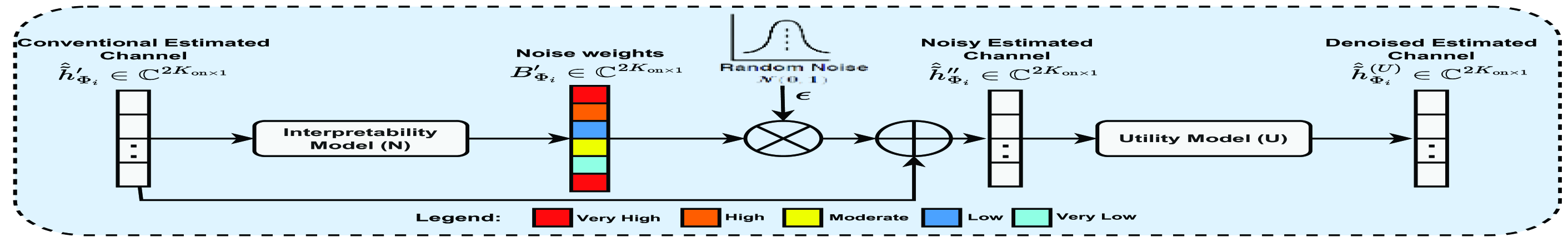
Fig. 2: Block diagram of the proposed XAI-CHEST scheme.

III-B TRFI-FNN

TRFI estimation scheme[15] is another methodology used for improving the DPA estimation in(4). Assuming that the time correlation of the channel response between two adjacent OFDM symbols is high, TRFI defines two sets of subcarriers such that: (i) ℛ⁢𝒮 i ℛ subscript 𝒮 𝑖{\mathcal{RS}}{i}caligraphic_R caligraphic_S start_POSTSUBSCRIPT italic_i end_POSTSUBSCRIPT set that includes the reliable subcarriers indices, and (ii) 𝒰⁢ℛ⁢𝒮 i 𝒰 ℛ subscript 𝒮 𝑖{\mathcal{URS}}{i}caligraphic_U caligraphic_R caligraphic_S start_POSTSUBSCRIPT italic_i end_POSTSUBSCRIPT set which contains the unreliable subcarriers indices. The estimated channels for 𝒰⁢ℛ⁢𝒮 i 𝒰 ℛ subscript 𝒮 𝑖{\mathcal{URS}}{i}caligraphic_U caligraphic_R caligraphic_S start_POSTSUBSCRIPT italic_i end_POSTSUBSCRIPT are then interpolated using the ℛ⁢𝒮 i ℛ subscript 𝒮 𝑖{\mathcal{RS}}{i}caligraphic_R caligraphic_S start_POSTSUBSCRIPT italic_i end_POSTSUBSCRIPT channel estimates by means of the frequency-domain cubic interpolation 1 1 1 The reliable/unreliable subcarriers are classified by TRFI channel estimator, while relevant/irrelevant subcarriers are classified by the proposed XAI scheme.. TRFI outperforms STA, especially in high SNR region. However, TRFI still suffers from demapping and interpolation errors, as the number of reliable subcarriers (RS) subcarriers is inversely proportional to the channel frequency selectivity. Therefore, applying cubic interpolation with only a few RS subcarriers degrades the performance. Therefore, an optimized FNN architecture is coined in[11] with 𝒉^TRFI i⁢[k]subscript^𝒉 subscript TRFI 𝑖 delimited-[]𝑘\hat{\tilde{\bm{h}}}{\text{TRFI}{i}}[k]over^ start_ARG over~ start_ARG bold_italic_h end_ARG end_ARG start_POSTSUBSCRIPT TRFI start_POSTSUBSCRIPT italic_i end_POSTSUBSCRIPT end_POSTSUBSCRIPT [ italic_k ] as an input instead of 𝒉^STA i⁢[k]subscript^𝒉 subscript STA 𝑖 delimited-[]𝑘\hat{\tilde{\bm{h}}}{\text{STA}{i}}[k]over^ start_ARG over~ start_ARG bold_italic_h end_ARG end_ARG start_POSTSUBSCRIPT STA start_POSTSUBSCRIPT italic_i end_POSTSUBSCRIPT end_POSTSUBSCRIPT [ italic_k ]. TRFI-FNN corrects the cubic interpolation error, thus leading to improved performance in high SNR regions. Since real-valued FNN model is considered, the conventional estimated channel should be converted from complex to real domain by stacking the real and imaginary parts of FNN input vector, where 𝒉^Φ i′∈ℝ 2⁢K on×1 subscript superscript^𝒉′subscript Φ 𝑖 superscript ℝ 2 subscript 𝐾 on 1\hat{\tilde{\bm{h}}}^{\prime}{\Phi{i}}\in\mathbb{R}^{2K_{\text{on}}\times 1}over^ start_ARG over~ start_ARG bold_italic_h end_ARG end_ARG start_POSTSUPERSCRIPT ′ end_POSTSUPERSCRIPT start_POSTSUBSCRIPT roman_Φ start_POSTSUBSCRIPT italic_i end_POSTSUBSCRIPT end_POSTSUBSCRIPT ∈ blackboard_R start_POSTSUPERSCRIPT 2 italic_K start_POSTSUBSCRIPT on end_POSTSUBSCRIPT × 1 end_POSTSUPERSCRIPT denotes the converted estimated channel vector, such that

𝒉^Φ i′=[ℜ⁡(𝒉^Φ i);ℑ⁡(𝒉^Φ i)]subscript superscript^𝒉′subscript Φ 𝑖 subscript^𝒉 subscript Φ 𝑖 subscript^𝒉 subscript Φ 𝑖\hat{\tilde{\bm{h}}}^{\prime}{\Phi{i}}=[\Re(\hat{\tilde{\bm{h}}}{\Phi{i}})% ;\Im(\hat{\tilde{\bm{h}}}{\Phi{i}})]over^ start_ARG over~ start_ARG bold_italic_h end_ARG end_ARG start_POSTSUPERSCRIPT ′ end_POSTSUPERSCRIPT start_POSTSUBSCRIPT roman_Φ start_POSTSUBSCRIPT italic_i end_POSTSUBSCRIPT end_POSTSUBSCRIPT = roman_ℜ ( over^ start_ARG over~ start_ARG bold_italic_h end_ARG end_ARG start_POSTSUBSCRIPT roman_Φ start_POSTSUBSCRIPT italic_i end_POSTSUBSCRIPT end_POSTSUBSCRIPT ) ; roman_ℑ ( over^ start_ARG over~ start_ARG bold_italic_h end_ARG end_ARG start_POSTSUBSCRIPT roman_Φ start_POSTSUBSCRIPT italic_i end_POSTSUBSCRIPT end_POSTSUBSCRIPT )

where 𝒉^Φ i∈ℂ K on×1 subscript^𝒉 subscript Φ 𝑖 superscript ℂ subscript 𝐾 on 1\hat{\tilde{\bm{h}}}{\Phi{i}}\in\mathbb{C}^{K_{\text{on}}\times 1}over^ start_ARG over~ start_ARG bold_italic_h end_ARG end_ARG start_POSTSUBSCRIPT roman_Φ start_POSTSUBSCRIPT italic_i end_POSTSUBSCRIPT end_POSTSUBSCRIPT ∈ blackboard_C start_POSTSUPERSCRIPT italic_K start_POSTSUBSCRIPT on end_POSTSUBSCRIPT × 1 end_POSTSUPERSCRIPT denotes the initially estimated channel and Φ∈[STA,TRFI]Φ delimited-[]STA,TRFI\Phi\in[\text{STA,\leavevmode\nobreak\ TRFI}]roman_Φ ∈ [ STA, TRFI ] refers to the estimation scheme.

IV Proposed XAI-CHEST Scheme

As discussed in the introduction, the interpretability of the black box model could be achieved either by studying its internal architecture or by externally analyzing the input-output relation. In this context, the proposed XAI-CHEST scheme provides a perturbation-based external interpretability of the black box channel estimation model, where the model inputs are classified as relevant and irrelevant. The main intuition is that if a subcarrier is relevant for the decision-making of a trained black box model, then adding noise with high weight to this subcarrier would negatively impact the accuracy of the model and vice-versa. Thus, it is expected that considering only the relevant subcarriers as model inputs would improve channel estimation performance. The methodology of the proposed XAI scheme is explained as follows.

Let U 𝑈 U italic_U be the utility model with parameters θ U subscript 𝜃 𝑈\theta_{U}italic_θ start_POSTSUBSCRIPT italic_U end_POSTSUBSCRIPT. The objective is to provide interpretability for the decisions taken by the U 𝑈 U italic_U model that refers to the black box model, i.e., STA-FNN or TRFI-FNN, in our case. We also define the interpretability noise model N 𝑁 N italic_N, with parameters θ N subscript 𝜃 𝑁\theta_{N}italic_θ start_POSTSUBSCRIPT italic_N end_POSTSUBSCRIPT, whose purpose is to compute the value of the induced noise weight to each subcarrier within the FNN input vector, i.e. 𝒉^STA i subscript^𝒉 subscript STA 𝑖\hat{\tilde{\bm{h}}}{\text{STA}{i}}over^ start_ARG over~ start_ARG bold_italic_h end_ARG end_ARG start_POSTSUBSCRIPT STA start_POSTSUBSCRIPT italic_i end_POSTSUBSCRIPT end_POSTSUBSCRIPT or 𝒉^TRFI i subscript^𝒉 subscript TRFI 𝑖\hat{\tilde{\bm{h}}}{\text{TRFI}{i}}over^ start_ARG over~ start_ARG bold_italic_h end_ARG end_ARG start_POSTSUBSCRIPT TRFI start_POSTSUBSCRIPT italic_i end_POSTSUBSCRIPT end_POSTSUBSCRIPT. The key idea lies in the customized loss function of the N 𝑁 N italic_N model that will adjust the induced noise while simultaneously maximizing the performance of the U 𝑈 U italic_U model. We note that both U 𝑈 U italic_U and N 𝑁 N italic_N models have the same FNN architecture, and the U 𝑈 U italic_U model is trained prior to the XAI processing, i.e., the weights of the U 𝑈 U italic_U model are frozen.

Let 𝒉^Φ i′∈ℝ 2⁢K on×1 subscript superscript^𝒉′subscript Φ 𝑖 superscript ℝ 2 subscript 𝐾 on 1\hat{\tilde{\bm{h}}}^{\prime}{\Phi{i}}\in\mathbb{R}^{2K_{\text{on}}\times 1}over^ start_ARG over~ start_ARG bold_italic_h end_ARG end_ARG start_POSTSUPERSCRIPT ′ end_POSTSUPERSCRIPT start_POSTSUBSCRIPT roman_Φ start_POSTSUBSCRIPT italic_i end_POSTSUBSCRIPT end_POSTSUBSCRIPT ∈ blackboard_R start_POSTSUPERSCRIPT 2 italic_K start_POSTSUBSCRIPT on end_POSTSUBSCRIPT × 1 end_POSTSUPERSCRIPT be the interpretability model input, where the latter produces a mask B Φ i′∈ℝ 2⁢K on×1 superscript subscript 𝐵 subscript Φ 𝑖′superscript ℝ 2 subscript 𝐾 on 1 B_{\Phi_{i}}^{\prime}\in\mathbb{R}^{2K_{\text{on}}\times 1}italic_B start_POSTSUBSCRIPT roman_Φ start_POSTSUBSCRIPT italic_i end_POSTSUBSCRIPT end_POSTSUBSCRIPT start_POSTSUPERSCRIPT ′ end_POSTSUPERSCRIPT ∈ blackboard_R start_POSTSUPERSCRIPT 2 italic_K start_POSTSUBSCRIPT on end_POSTSUBSCRIPT × 1 end_POSTSUPERSCRIPT that can be represented as follows

B Φ i′=N⁢(𝒉^Φ i′,θ N)superscript subscript 𝐵 subscript Φ 𝑖′𝑁 subscript superscript^𝒉′subscript Φ 𝑖 subscript 𝜃 𝑁 B_{\Phi_{i}}^{\prime}=N(\hat{\tilde{\bm{h}}}^{\prime}{\Phi{i}},\theta_{N})italic_B start_POSTSUBSCRIPT roman_Φ start_POSTSUBSCRIPT italic_i end_POSTSUBSCRIPT end_POSTSUBSCRIPT start_POSTSUPERSCRIPT ′ end_POSTSUPERSCRIPT = italic_N ( over^ start_ARG over~ start_ARG bold_italic_h end_ARG end_ARG start_POSTSUPERSCRIPT ′ end_POSTSUPERSCRIPT start_POSTSUBSCRIPT roman_Φ start_POSTSUBSCRIPT italic_i end_POSTSUBSCRIPT end_POSTSUBSCRIPT , italic_θ start_POSTSUBSCRIPT italic_N end_POSTSUBSCRIPT )(8)

where B Φ i′∈[0,1]superscript subscript 𝐵 subscript Φ 𝑖′0 1 B_{\Phi_{i}}^{\prime}\in[0,1]italic_B start_POSTSUBSCRIPT roman_Φ start_POSTSUBSCRIPT italic_i end_POSTSUBSCRIPT end_POSTSUBSCRIPT start_POSTSUPERSCRIPT ′ end_POSTSUPERSCRIPT ∈ [ 0 , 1 ] determines the weight of noise applied to each element in 𝒉^Φ i′subscript superscript^𝒉′subscript Φ 𝑖\hat{\tilde{\bm{h}}}^{\prime}{\Phi{i}}over^ start_ARG over~ start_ARG bold_italic_h end_ARG end_ARG start_POSTSUPERSCRIPT ′ end_POSTSUPERSCRIPT start_POSTSUBSCRIPT roman_Φ start_POSTSUBSCRIPT italic_i end_POSTSUBSCRIPT end_POSTSUBSCRIPT. We note that the scaling of B Φ i′superscript subscript 𝐵 subscript Φ 𝑖′B_{\Phi_{i}}^{\prime}italic_B start_POSTSUBSCRIPT roman_Φ start_POSTSUBSCRIPT italic_i end_POSTSUBSCRIPT end_POSTSUBSCRIPT start_POSTSUPERSCRIPT ′ end_POSTSUPERSCRIPT is achieved by using the sigmoid activation function. Based on B Φ i′superscript subscript 𝐵 subscript Φ 𝑖′B_{\Phi_{i}}^{\prime}italic_B start_POSTSUBSCRIPT roman_Φ start_POSTSUBSCRIPT italic_i end_POSTSUBSCRIPT end_POSTSUBSCRIPT start_POSTSUPERSCRIPT ′ end_POSTSUPERSCRIPT, the conventional estimated channel vector including the induced noise 𝒉^Φ i′′subscript superscript^𝒉′′subscript Φ 𝑖\hat{\tilde{\bm{h}}}^{\prime\prime}{\Phi{i}}over^ start_ARG over~ start_ARG bold_italic_h end_ARG end_ARG start_POSTSUPERSCRIPT ′ ′ end_POSTSUPERSCRIPT start_POSTSUBSCRIPT roman_Φ start_POSTSUBSCRIPT italic_i end_POSTSUBSCRIPT end_POSTSUBSCRIPT can be expressed such that

𝒉^Φ i′′=𝒉^Φ i′+B Φ i′⁢ϵ subscript superscript^𝒉′′subscript Φ 𝑖 subscript superscript^𝒉′subscript Φ 𝑖 superscript subscript 𝐵 subscript Φ 𝑖′italic-ϵ\hat{\tilde{\bm{h}}}^{\prime\prime}{\Phi{i}}=\hat{\tilde{\bm{h}}}^{\prime}{% \Phi{i}}+B_{\Phi_{i}}^{\prime}\epsilon over^ start_ARG over~ start_ARG bold_italic_h end_ARG end_ARG start_POSTSUPERSCRIPT ′ ′ end_POSTSUPERSCRIPT start_POSTSUBSCRIPT roman_Φ start_POSTSUBSCRIPT italic_i end_POSTSUBSCRIPT end_POSTSUBSCRIPT = over^ start_ARG over~ start_ARG bold_italic_h end_ARG end_ARG start_POSTSUPERSCRIPT ′ end_POSTSUPERSCRIPT start_POSTSUBSCRIPT roman_Φ start_POSTSUBSCRIPT italic_i end_POSTSUBSCRIPT end_POSTSUBSCRIPT + italic_B start_POSTSUBSCRIPT roman_Φ start_POSTSUBSCRIPT italic_i end_POSTSUBSCRIPT end_POSTSUBSCRIPT start_POSTSUPERSCRIPT ′ end_POSTSUPERSCRIPT italic_ϵ(9)

Here, ϵ∼𝒩⁢(0,1)similar-to italic-ϵ 𝒩 0 1\epsilon\sim\mathcal{N}(0,1)italic_ϵ ∼ caligraphic_N ( 0 , 1 ) denotes the random noise sampled from the standard normal distribution. After that, 𝒉^Φ i′′subscript superscript^𝒉′′subscript Φ 𝑖\hat{\tilde{\bm{h}}}^{\prime\prime}{\Phi{i}}over^ start_ARG over~ start_ARG bold_italic_h end_ARG end_ARG start_POSTSUPERSCRIPT ′ ′ end_POSTSUPERSCRIPT start_POSTSUBSCRIPT roman_Φ start_POSTSUBSCRIPT italic_i end_POSTSUBSCRIPT end_POSTSUBSCRIPT is fed as input to the frozen utility model U 𝑈 U italic_U, i.e, STA-FNN or TRFI-FNN, such that

𝒉^Φ i(U)=U⁢(𝒉^Φ i′′,θ U)subscript superscript^𝒉 U subscript Φ 𝑖 𝑈 subscript superscript^𝒉′′subscript Φ 𝑖 subscript 𝜃 𝑈\hat{\tilde{\bm{h}}}^{(\text{U})}{\Phi{i}}=U(\hat{\tilde{\bm{h}}}^{\prime% \prime}{\Phi{i}},\theta_{U})over^ start_ARG over~ start_ARG bold_italic_h end_ARG end_ARG start_POSTSUPERSCRIPT ( U ) end_POSTSUPERSCRIPT start_POSTSUBSCRIPT roman_Φ start_POSTSUBSCRIPT italic_i end_POSTSUBSCRIPT end_POSTSUBSCRIPT = italic_U ( over^ start_ARG over~ start_ARG bold_italic_h end_ARG end_ARG start_POSTSUPERSCRIPT ′ ′ end_POSTSUPERSCRIPT start_POSTSUBSCRIPT roman_Φ start_POSTSUBSCRIPT italic_i end_POSTSUBSCRIPT end_POSTSUBSCRIPT , italic_θ start_POSTSUBSCRIPT italic_U end_POSTSUBSCRIPT )(10)

The aim of training the interpretability model is to minimize the following customized loss function:

L N=min θ N⁡[L U−λ⁢log⁡(B Φ i′)]subscript L N subscript subscript 𝜃 N subscript L U 𝜆 superscript subscript B subscript Φ i′\pazocal{L}{N}=\min{\theta_{N}}\big{[}\pazocal{L}{U}-\lambda\log(B{\Phi_{i% }}^{\prime})\big{]}roman_L start_POSTSUBSCRIPT roman_N end_POSTSUBSCRIPT = roman_min start_POSTSUBSCRIPT italic_θ start_POSTSUBSCRIPT roman_N end_POSTSUBSCRIPT end_POSTSUBSCRIPT roman_L start_POSTSUBSCRIPT roman_U end_POSTSUBSCRIPT - italic_λ roman_log ( roman_B start_POSTSUBSCRIPT roman_Φ start_POSTSUBSCRIPT roman_i end_POSTSUBSCRIPT end_POSTSUBSCRIPT start_POSTSUPERSCRIPT ′ end_POSTSUPERSCRIPT )

The first term in Eq. (11) is the loss function of the utility model U 𝑈 U italic_U that represents mean squared error (MSE) between the initially estimated channel 𝒉^Φ i′subscript superscript^𝒉′subscript Φ 𝑖\hat{\tilde{\bm{h}}}^{\prime}{\Phi{i}}over^ start_ARG over~ start_ARG bold_italic_h end_ARG end_ARG start_POSTSUPERSCRIPT ′ end_POSTSUPERSCRIPT start_POSTSUBSCRIPT roman_Φ start_POSTSUBSCRIPT italic_i end_POSTSUBSCRIPT end_POSTSUBSCRIPT and the true channel 𝒉Φ i subscript𝒉 subscript Φ 𝑖{\tilde{\bm{h}}}{\Phi{i}}over~ start_ARG bold_italic_h end_ARG start_POSTSUBSCRIPT roman_Φ start_POSTSUBSCRIPT italic_i end_POSTSUBSCRIPT end_POSTSUBSCRIPT, such that:

L U=1 N t⁢r.∑i=1 N t⁢r(𝐡Φ i−𝐡^Φ i′)2 formulae-sequence subscript L U 1 subscript N t r superscript subscript i 1 subscript N t r superscript subscript𝐡 subscript Φ i subscript superscript^𝐡′subscript Φ i 2\pazocal{L}{U}=\frac{1}{N{tr}}.\sum_{i=1}^{N_{tr}}\big{(}{\tilde{\bm{h}}}{% \Phi{i}}-\hat{\tilde{\bm{h}}}^{\prime}{\Phi{i}}\big{)}^{2}roman_L start_POSTSUBSCRIPT roman_U end_POSTSUBSCRIPT = divide start_ARG 1 end_ARG start_ARG roman_N start_POSTSUBSCRIPT roman_t roman_r end_POSTSUBSCRIPT end_ARG . ∑ start_POSTSUBSCRIPT roman_i = 1 end_POSTSUBSCRIPT start_POSTSUPERSCRIPT roman_N start_POSTSUBSCRIPT roman_t roman_r end_POSTSUBSCRIPT end_POSTSUPERSCRIPT ( over~ start_ARG bold_h end_ARG start_POSTSUBSCRIPT roman_Φ start_POSTSUBSCRIPT roman_i end_POSTSUBSCRIPT end_POSTSUBSCRIPT - over^ start_ARG over~ start_ARG bold_h end_ARG end_ARG start_POSTSUPERSCRIPT ′ end_POSTSUPERSCRIPT start_POSTSUBSCRIPT roman_Φ start_POSTSUBSCRIPT roman_i end_POSTSUBSCRIPT end_POSTSUBSCRIPT ) start_POSTSUPERSCRIPT 2 end_POSTSUPERSCRIPT(12)

where N t⁢r subscript 𝑁 𝑡 𝑟 N_{tr}italic_N start_POSTSUBSCRIPT italic_t italic_r end_POSTSUBSCRIPT is the number of training samples used. The second term in(11) boosts the growth of the noise weight for each element in 𝒉^Φ i′′subscript superscript^𝒉′′subscript Φ 𝑖\hat{\tilde{\bm{h}}}^{\prime\prime}{\Phi{i}}over^ start_ARG over~ start_ARG bold_italic_h end_ARG end_ARG start_POSTSUPERSCRIPT ′ ′ end_POSTSUPERSCRIPT start_POSTSUBSCRIPT roman_Φ start_POSTSUBSCRIPT italic_i end_POSTSUBSCRIPT end_POSTSUBSCRIPT so that relevant and irrelevant subcarriers can be identified. We would like to mention that the training of the interpretability model N 𝑁 N italic_N is performed once according to the channel model used. In the testing phase, the obtained B Φ i′superscript subscript 𝐵 subscript Φ 𝑖′B_{\Phi_{i}}^{\prime}italic_B start_POSTSUBSCRIPT roman_Φ start_POSTSUBSCRIPT italic_i end_POSTSUBSCRIPT end_POSTSUBSCRIPT start_POSTSUPERSCRIPT ′ end_POSTSUPERSCRIPT includes the noise weights for the real and imaginary parts of each input subcarrier. B Φ i′superscript subscript 𝐵 subscript Φ 𝑖′B_{\Phi_{i}}^{\prime}italic_B start_POSTSUBSCRIPT roman_Φ start_POSTSUBSCRIPT italic_i end_POSTSUBSCRIPT end_POSTSUBSCRIPT start_POSTSUPERSCRIPT ′ end_POSTSUPERSCRIPT is scaled back to B Φ i∈ℝ K on×1 subscript 𝐵 subscript Φ 𝑖 superscript ℝ subscript 𝐾 on 1 B_{\Phi_{i}}\in\mathbb{R}^{K_{\text{on}}\times 1}italic_B start_POSTSUBSCRIPT roman_Φ start_POSTSUBSCRIPT italic_i end_POSTSUBSCRIPT end_POSTSUBSCRIPT ∈ blackboard_R start_POSTSUPERSCRIPT italic_K start_POSTSUBSCRIPT on end_POSTSUBSCRIPT × 1 end_POSTSUPERSCRIPT, where the noise weight of the real and imaginary parts for each subcarrier are averaged. The motivation behind this averaging lies in the fact that it is noticed during the training phase that the interpretability model produces almost the same noise weight for the real and imaging parts of each subcarrier within 𝒉^Φ i′subscript superscript^𝒉′subscript Φ 𝑖\hat{\tilde{\bm{h}}}^{\prime}{\Phi{i}}over^ start_ARG over~ start_ARG bold_italic_h end_ARG end_ARG start_POSTSUPERSCRIPT ′ end_POSTSUPERSCRIPT start_POSTSUBSCRIPT roman_Φ start_POSTSUBSCRIPT italic_i end_POSTSUBSCRIPT end_POSTSUBSCRIPT. Figure2 shows the block diagram of the proposed XAI-CHEST scheme.

Algorithm1 illustrates the training process of the interpretability model (N). 𝑯^Φ′∈ℝ 2⁢K on×I tr subscript superscript^𝑯′Φ superscript ℝ 2 subscript 𝐾 on subscript 𝐼 tr\hat{\tilde{\bm{H}}}^{\prime}{\Phi}\in\mathbb{R}^{2K{\text{on}}\times I_{% \text{tr}}}over^ start_ARG over~ start_ARG bold_italic_H end_ARG end_ARG start_POSTSUPERSCRIPT ′ end_POSTSUPERSCRIPT start_POSTSUBSCRIPT roman_Φ end_POSTSUBSCRIPT ∈ blackboard_R start_POSTSUPERSCRIPT 2 italic_K start_POSTSUBSCRIPT on end_POSTSUBSCRIPT × italic_I start_POSTSUBSCRIPT tr end_POSTSUBSCRIPT end_POSTSUPERSCRIPT and 𝑯Φ∈ℝ 2⁢K on×I tr subscript𝑯 Φ superscript ℝ 2 subscript 𝐾 on subscript 𝐼 tr{\tilde{\bm{H}}}{\Phi}\in\mathbb{R}^{2K{\text{on}}\times I_{\text{tr}}}over~ start_ARG bold_italic_H end_ARG start_POSTSUBSCRIPT roman_Φ end_POSTSUBSCRIPT ∈ blackboard_R start_POSTSUPERSCRIPT 2 italic_K start_POSTSUBSCRIPT on end_POSTSUBSCRIPT × italic_I start_POSTSUBSCRIPT tr end_POSTSUBSCRIPT end_POSTSUPERSCRIPT denote the training dataset pairs of the conventional estimated channels and the true ones, where I tr subscript 𝐼 tr I_{\text{tr}}italic_I start_POSTSUBSCRIPT tr end_POSTSUBSCRIPT is the size of the training dataset.

Algorithm 1 Interpretability model (N) training

0:Estimated channel:

𝑯^Φ′subscript superscript^𝑯′Φ\hat{\tilde{\bm{H}}}^{\prime}_{\Phi}over^ start_ARG over~ start_ARG bold_italic_H end_ARG end_ARG start_POSTSUPERSCRIPT ′ end_POSTSUPERSCRIPT start_POSTSUBSCRIPT roman_Φ end_POSTSUBSCRIPT , true channel:

𝑯Φ subscript𝑯 Φ{\tilde{\bm{H}}}_{\Phi}over~ start_ARG bold_italic_H end_ARG start_POSTSUBSCRIPT roman_Φ end_POSTSUBSCRIPT , learning rate:

η 𝜂\eta italic_η , trained utility model

U 𝑈 U italic_U with parameters

θ U subscript 𝜃 𝑈\theta_{U}italic_θ start_POSTSUBSCRIPT italic_U end_POSTSUBSCRIPT

0:Trained interpretability model (N) with parameters

θ N subscript 𝜃 𝑁\theta_{N}italic_θ start_POSTSUBSCRIPT italic_N end_POSTSUBSCRIPT

while not converged do

for

𝒉^Φ i′∈𝑯^Φ i′subscript superscript^𝒉′subscript Φ 𝑖 subscript superscript^𝑯′subscript Φ 𝑖\hat{\tilde{\bm{h}}}^{\prime}{\Phi{i}}\in\hat{\tilde{\bm{H}}}^{\prime}_{\Phi% _{i}}over^ start_ARG over~ start_ARG bold_italic_h end_ARG end_ARG start_POSTSUPERSCRIPT ′ end_POSTSUPERSCRIPT start_POSTSUBSCRIPT roman_Φ start_POSTSUBSCRIPT italic_i end_POSTSUBSCRIPT end_POSTSUBSCRIPT ∈ over^ start_ARG over~ start_ARG bold_italic_H end_ARG end_ARG start_POSTSUPERSCRIPT ′ end_POSTSUPERSCRIPT start_POSTSUBSCRIPT roman_Φ start_POSTSUBSCRIPT italic_i end_POSTSUBSCRIPT end_POSTSUBSCRIPT ,

𝒉Φ i∈𝑯Φ i subscript𝒉 subscript Φ 𝑖 subscript𝑯 subscript Φ 𝑖{\tilde{\bm{h}}}{\Phi{i}}\in{\tilde{\bm{H}}}{\Phi{i}}over~ start_ARG bold_italic_h end_ARG start_POSTSUBSCRIPT roman_Φ start_POSTSUBSCRIPT italic_i end_POSTSUBSCRIPT end_POSTSUBSCRIPT ∈ over~ start_ARG bold_italic_H end_ARG start_POSTSUBSCRIPT roman_Φ start_POSTSUBSCRIPT italic_i end_POSTSUBSCRIPT end_POSTSUBSCRIPT do

B Φ i′superscript subscript 𝐵 subscript Φ 𝑖′B_{\Phi_{i}}^{\prime}italic_B start_POSTSUBSCRIPT roman_Φ start_POSTSUBSCRIPT italic_i end_POSTSUBSCRIPT end_POSTSUBSCRIPT start_POSTSUPERSCRIPT ′ end_POSTSUPERSCRIPT←←\leftarrow←N⁢(𝒉^Φ i′,θ N)𝑁 subscript superscript^𝒉′subscript Φ 𝑖 subscript 𝜃 𝑁 N(\hat{\tilde{\bm{h}}}^{\prime}{\Phi{i}},\theta_{N})italic_N ( over^ start_ARG over~ start_ARG bold_italic_h end_ARG end_ARG start_POSTSUPERSCRIPT ′ end_POSTSUPERSCRIPT start_POSTSUBSCRIPT roman_Φ start_POSTSUBSCRIPT italic_i end_POSTSUBSCRIPT end_POSTSUBSCRIPT , italic_θ start_POSTSUBSCRIPT italic_N end_POSTSUBSCRIPT )

ϵ italic-ϵ\epsilon italic_ϵ←←\leftarrow←𝒩⁢(0,1)𝒩 0 1\mathcal{N}(0,1)caligraphic_N ( 0 , 1 )

𝒉^Φ i′′subscript superscript^𝒉′′subscript Φ 𝑖\hat{\tilde{\bm{h}}}^{\prime\prime}{\Phi{i}}over^ start_ARG over~ start_ARG bold_italic_h end_ARG end_ARG start_POSTSUPERSCRIPT ′ ′ end_POSTSUPERSCRIPT start_POSTSUBSCRIPT roman_Φ start_POSTSUBSCRIPT italic_i end_POSTSUBSCRIPT end_POSTSUBSCRIPT←←\leftarrow←𝒉^Φ i′+B Φ i′⁢ϵ subscript superscript^𝒉′subscript Φ 𝑖 superscript subscript 𝐵 subscript Φ 𝑖′italic-ϵ\hat{\tilde{\bm{h}}}^{\prime}{\Phi{i}}+B_{\Phi_{i}}^{\prime}\epsilon over^ start_ARG over~ start_ARG bold_italic_h end_ARG end_ARG start_POSTSUPERSCRIPT ′ end_POSTSUPERSCRIPT start_POSTSUBSCRIPT roman_Φ start_POSTSUBSCRIPT italic_i end_POSTSUBSCRIPT end_POSTSUBSCRIPT + italic_B start_POSTSUBSCRIPT roman_Φ start_POSTSUBSCRIPT italic_i end_POSTSUBSCRIPT end_POSTSUBSCRIPT start_POSTSUPERSCRIPT ′ end_POSTSUPERSCRIPT italic_ϵ

𝒉^Φ i(U)subscript superscript^𝒉 U subscript Φ 𝑖\hat{\tilde{\bm{h}}}^{(\text{U})}{\Phi{i}}over^ start_ARG over~ start_ARG bold_italic_h end_ARG end_ARG start_POSTSUPERSCRIPT ( U ) end_POSTSUPERSCRIPT start_POSTSUBSCRIPT roman_Φ start_POSTSUBSCRIPT italic_i end_POSTSUBSCRIPT end_POSTSUBSCRIPT←←\leftarrow←U⁢(𝒉^Φ i′′,θ U)𝑈 subscript superscript^𝒉′′subscript Φ 𝑖 subscript 𝜃 𝑈 U(\hat{\tilde{\bm{h}}}^{\prime\prime}{\Phi{i}},\theta_{U})italic_U ( over^ start_ARG over~ start_ARG bold_italic_h end_ARG end_ARG start_POSTSUPERSCRIPT ′ ′ end_POSTSUPERSCRIPT start_POSTSUBSCRIPT roman_Φ start_POSTSUBSCRIPT italic_i end_POSTSUBSCRIPT end_POSTSUBSCRIPT , italic_θ start_POSTSUBSCRIPT italic_U end_POSTSUBSCRIPT )

L U subscript L U\pazocal{L}{U}roman_L start_POSTSUBSCRIPT roman_U end_POSTSUBSCRIPT←←\leftarrow←MSE⁢(𝒉Φ i−𝒉^Φ i(U))MSE subscript𝒉 subscript Φ 𝑖 subscript superscript^𝒉 U subscript Φ 𝑖\text{MSE}\big{(}{\tilde{\bm{h}}}{\Phi_{i}}-\hat{\tilde{\bm{h}}}^{(\text{U})}% {\Phi{i}}\big{)}MSE ( over~ start_ARG bold_italic_h end_ARG start_POSTSUBSCRIPT roman_Φ start_POSTSUBSCRIPT italic_i end_POSTSUBSCRIPT end_POSTSUBSCRIPT - over^ start_ARG over~ start_ARG bold_italic_h end_ARG end_ARG start_POSTSUPERSCRIPT ( U ) end_POSTSUPERSCRIPT start_POSTSUBSCRIPT roman_Φ start_POSTSUBSCRIPT italic_i end_POSTSUBSCRIPT end_POSTSUBSCRIPT )

L N subscript L N\pazocal{L}{N}roman_L start_POSTSUBSCRIPT roman_N end_POSTSUBSCRIPT←←\leftarrow←L U subscript L U\pazocal{L}{U}roman_L start_POSTSUBSCRIPT roman_U end_POSTSUBSCRIPT−λ⁢log⁡(B Φ i′)𝜆 superscript subscript 𝐵 subscript Φ 𝑖′-\lambda\log(B_{\Phi_{i}}^{\prime})- italic_λ roman_log ( italic_B start_POSTSUBSCRIPT roman_Φ start_POSTSUBSCRIPT italic_i end_POSTSUBSCRIPT end_POSTSUBSCRIPT start_POSTSUPERSCRIPT ′ end_POSTSUPERSCRIPT )

θ N subscript 𝜃 𝑁\theta_{N}italic_θ start_POSTSUBSCRIPT italic_N end_POSTSUBSCRIPT←←\leftarrow←θ N+η⁢∂L N∂θ N subscript 𝜃 𝑁 𝜂 subscript L N subscript 𝜃 𝑁\theta_{N}+\eta\frac{\partial\pazocal{L}{N}}{\partial\theta{N}}italic_θ start_POSTSUBSCRIPT italic_N end_POSTSUBSCRIPT + italic_η divide start_ARG ∂ roman_L start_POSTSUBSCRIPT roman_N end_POSTSUBSCRIPT end_ARG start_ARG ∂ italic_θ start_POSTSUBSCRIPT italic_N end_POSTSUBSCRIPT end_ARG

end for

end while

V Simulation Results

(a) Low frequency-selective vehicular channel model.

(b) High frequency-selective vehicular channel model.

Fig. 3: BER Performance for high mobility vehicular channel models.

(a) Low frequency-selective vehicular channel model.

(b) High frequency-selective vehicular channel model.

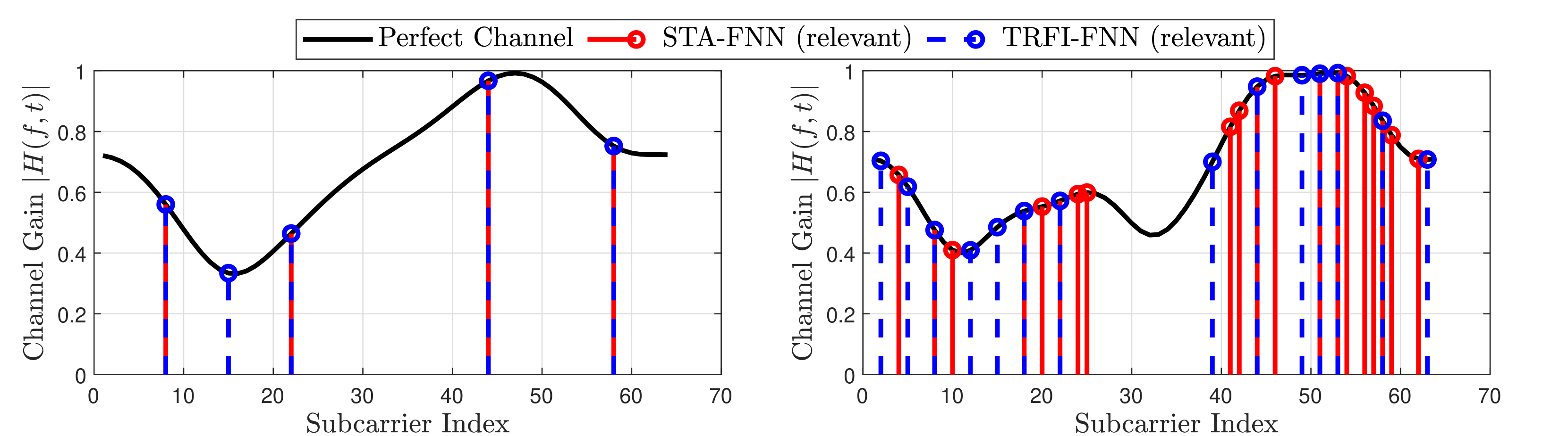
Fig. 4: Selected relevant subcarriers by the proposed interpretability model.

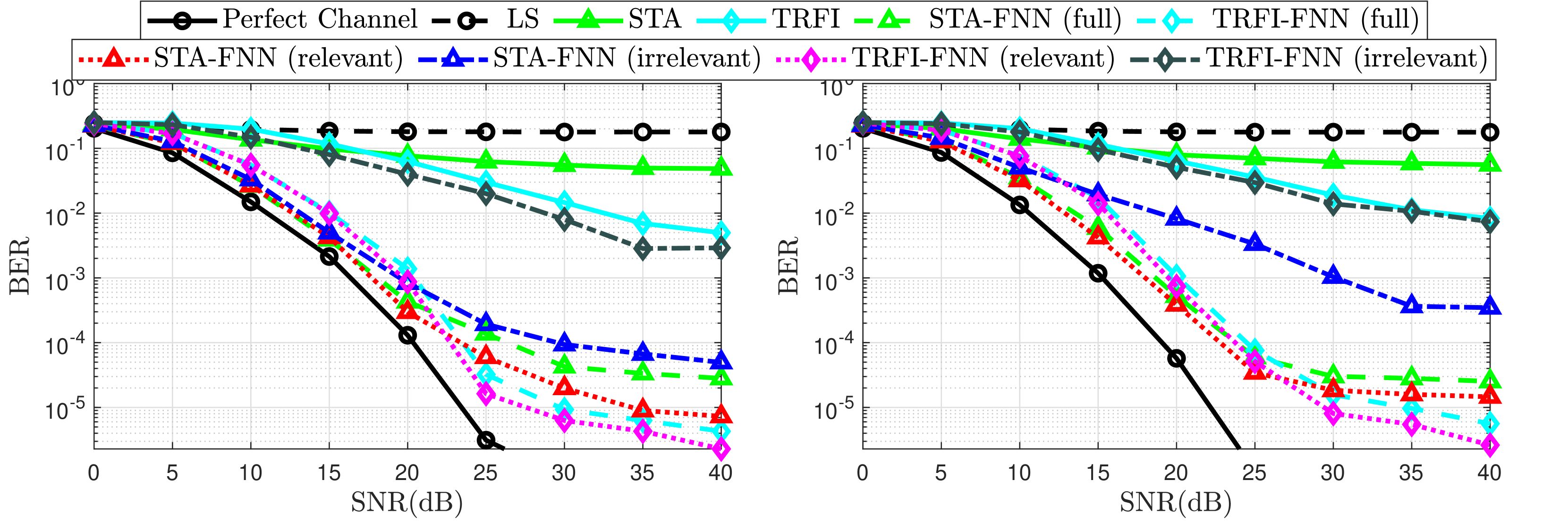
This section illustrates the performance evaluation of the proposed XAI-CHEST scheme, where BER performance of STA-FNN and TRFI-FNN estimators is analyzed taking into consideration full, relevant, and irrelevant subcarriers. We note that the noise thresholds used to classify the subcarriers are empirically chosen and defined as N TRFI-th=0.6 subscript 𝑁 TRFI-th 0.6 N_{\text{TRFI-th}}=0.6 italic_N start_POSTSUBSCRIPT TRFI-th end_POSTSUBSCRIPT = 0.6 and N STA-th=0.3 subscript 𝑁 STA-th 0.3 N_{\text{STA-th}}=0.3 italic_N start_POSTSUBSCRIPT STA-th end_POSTSUBSCRIPT = 0.3, where the systematic fine-tuning of them is kept as future work. This means that all the subcarriers given a noise weight greater than the defined threshold are classified as irrelevant subcarriers and vice-versa.

BER is evaluated using two vehicular channel models[16] as shown in TableI: (i) Low-frequency selectivity, where Vehicle-to-Vehicle urban scenario (VTV-US) is employed. (ii) High-frequency selectivity, where Vehicle-to-Infrastructure urban scenario (VTI-US) is considered. In both scenarios, Doppler frequency f d=1000 subscript 𝑓 𝑑 1000 f_{d}=1000 italic_f start_POSTSUBSCRIPT italic_d end_POSTSUBSCRIPT = 1000 Hz is considered. Both the interpretability and utility models are trained using a 100,000 100 000 100,000 100 , 000 OFDM symbols dataset, splitted into 80%percent 80 80%80 % training and 20%percent 20 20%20 % testing. ADAM optimizer is used with a learning rate l⁢r=0.001 𝑙 𝑟 0.001 lr=0.001 italic_l italic_r = 0.001 with batch size equals 128 128 128 128 for 500 500 500 500 epoch. Simulation parameters are based on the IEEE 802.11p standard[8], where the comb pilot allocation is used so that K p=4 subscript 𝐾 𝑝 4 K_{p}=4 italic_K start_POSTSUBSCRIPT italic_p end_POSTSUBSCRIPT = 4, K d=48 subscript 𝐾 𝑑 48 K_{d}=48 italic_K start_POSTSUBSCRIPT italic_d end_POSTSUBSCRIPT = 48, K n=12 subscript 𝐾 𝑛 12 K_{n}=12 italic_K start_POSTSUBSCRIPT italic_n end_POSTSUBSCRIPT = 12, and I=50 𝐼 50 I=50 italic_I = 50. QPSK modulation is considered with SNR ranges [0,5,…,40]0 5…40[0,5,\dots,40][ 0 , 5 , … , 40 ] dB.

Table I: Characteristics of the employed channel models following Jake’s Doppler spectrum.

Figure3 depicts the BER performance of the STA-FNN and TRFI-FNN channel estimation schemes studied. It is clearly shown that employing only the LS channel estimation suffers from severe performance degradation, as the channel becomes outdated among the received OFDM symbols. Moreover, limited improvement can be achieved with the conventional STA and TRFI channel estimation scheme due to the enlarged DPA demapping error. This is attributed to the fact that conventional STA estimation outperforms TRFI in low SNR regions because of frequency and time averaging operations that can alleviate the impact of noise and demapping error in low SNR regions. However, the averaging operations are not useful in high SNR regions since the impact of noise is low, and the STA averaging coefficients are fixed. Hence, the TRFI channel estimation is more accurate in high SNR regions. As observed, FNN can implicitly learn the channel correlations apart from preventing a high demapping error arising from conventional estimation where STA-FNN and TRFI-FNN significantly outperform conventional STA and TRFI estimators.

In order to evaluate the performance of the proposed XAI-CHEST scheme, both STA-FNN and TRFI-FNN estimators are implemented in three different configurations: (i) Full where 𝒉^Φ i′∈ℝ 2⁢K on×1 subscript superscript^𝒉′subscript Φ 𝑖 superscript ℝ 2 subscript 𝐾 on 1\hat{\tilde{\bm{h}}}^{\prime}{\Phi{i}}\in\mathbb{R}^{2K_{\text{on}}\times 1}over^ start_ARG over~ start_ARG bold_italic_h end_ARG end_ARG start_POSTSUPERSCRIPT ′ end_POSTSUPERSCRIPT start_POSTSUBSCRIPT roman_Φ start_POSTSUBSCRIPT italic_i end_POSTSUBSCRIPT end_POSTSUBSCRIPT ∈ blackboard_R start_POSTSUPERSCRIPT 2 italic_K start_POSTSUBSCRIPT on end_POSTSUBSCRIPT × 1 end_POSTSUPERSCRIPT includes all sub-carriers as an FNN input. (ii) Relevant where only relevant subcarriers experiencing noise below the defined N Φ⁢-th subscript 𝑁 Φ-th N_{\Phi\text{-th}}italic_N start_POSTSUBSCRIPT roman_Φ -th end_POSTSUBSCRIPT are fed to the FNN. (ii) Irrelevant where irrelevant subcarriers recording noise weights above the defined threshold are considered. It is worth mentioning that when the relevant subcarriers are used instead of the full subcarriers, STA-FNN and TRFI-FNN perform better and 2 2 2 2 dB and 1 1 1 1 dB gain are achieved in terms of SNR for BER =10−4 absent superscript 10 4=10^{-4}= 10 start_POSTSUPERSCRIPT - 4 end_POSTSUPERSCRIPT, respectively. On the contrary, significant performance degradation can be noticed for both STA-FNN and TRFI-NN estimators when irrelevant subcarriers are used, even though the number of irrelevant subcarriers is greater than the number of relevant subcarriers 2 2 2 BER is computed over all the data subcarriers within the received OFDM symbols. The difference lies in the size of the FNN input vector that includes the relevant or irrelevant subcarriers..

In order to further validate the recorded BER results, the position of relevant subcarriers selected by the interpretability model is analyzed, as illustrated in Figure4. It is clearly shown that the relevant subcarriers experiencing low noise induced by the interpretability model are distributed among the sharp channel variations. This reveals that it is not necessary for the FNN model to have the full K o⁢n=52 subscript 𝐾 𝑜 𝑛 52 K_{on}=52 italic_K start_POSTSUBSCRIPT italic_o italic_n end_POSTSUBSCRIPT = 52 subcarriers as an input. It can perform better by choosing the appropriate subcarriers to capture the main channel variation among the subcarriers. Moreover, the number of selected relevant subcarriers increases with the increase in frequency selectivity. In high-frequency selectivity, the channel variation across the subcarriers becomes more challenging, and thus more subcarriers are required by the FNN to accurately estimate the channel. Moreover, it can be noticed that as the accuracy of the initial estimation increases, the number of selected relevant subcarriers decreases, where STA-FNN requires more relevant subcarriers than TRFI-FNN. This means that the interpretability model is able to induce more noise weight to the irrelevant subcarriers within TRFI-FNN since it is more accurate, whereas less noise is induced to the STA-FNN input since it is already noisy. Finally, fine-tuning the noise threshold can be achieved by studying the characteristics of the channel model employed and the BER requirement. However, in all cases, using the proposed XAI-CHEST scheme provides a reasonable interpretation of the behavior of the employed FNN black-box model. In addition, selecting the relevant FNN inputs leads to improving the BER performance as well as decreasing the computational complexity due to optimizing the FNN input and the FNN architecture accordingly.

VI Conclusion

Building trust and transparency of the AI-based solution is a critical issue in future 6G communications. The need to provide reasonable interpretability of the black box AI models is a must. In this context, an XAI-CHEST scheme is proposed where the interpretability of the recently proposed FNN-based channel estimation schemes is thoroughly investigated. The proposed XAI-CHEST scheme aims to induce higher noise weights on the irrelevant FNN input subcarriers, thus, enabling a trustworthy, optimized, and robust channel estimation. Simulation results reveal that employing only the relevant subcarriers within the channel estimation leads to a significant improvement in the BER performance while optimizing the FNN input. Therefore, ensuring that FNN models are able to learn the most relevant features that maximize the channel estimation accuracy, as well as, reducing the computational complexity of the FNN-based channel estimators. It is worth mentioning that the proposed XAI methodology can be easily adapted to any application other than channel estimation. As a future perspective, performance improvement using several pilot pattern designs according to the generated noise weights will be studied. In addition, the possibility of optimizing the FNN architecture based on the reduced input size as well as the required inference time will be investigated.

References

• [1] W.Guo, “Explainable Artificial Intelligence for 6G: Improving Trust between Human and Machine,” IEEE Communications Magazine, vol.58, no.6, pp. 39–45, 2020.
• [2] R.S. Balan, S.Deepa, and C.Balakrishnan, “Transforming Towards 6G: Critical Review of Key Performance Indicators,” in 2022 4th International Conference on Circuits, Control, Communication and Computing (I4C), 2022, pp. 341–346.
• [3] M.Zolanvari, Z.Yang, K.Khan, R.Jain, and N.Meskin, “TRUST XAI: Model-Agnostic Explanations for AI With a Case Study on IIoT Security,” IEEE Internet of Things Journal, vol.10, no.4, pp. 2967–2978, 2023.
• [4] N.Khan, S.Coleri, A.Abdallah, A.Celik, and A.M. Eltawil, “Explainable and Robust Artificial Intelligence for Trustworthy Resource Management in 6G Networks,” IEEE Communications Magazine, pp. 1–7, 2023.
• [5] Y.Yang, F.Gao, X.Ma, and S.Zhang, “Deep Learning-Based Channel Estimation for Doubly Selective Fading Channels,” IEEE Access, vol.7, pp. 36 579–36 589, 2019.
• [6] A.Loquercio, M.Segu, and D.Scaramuzza, “A General Framework for Uncertainty Estimation in Deep Learning,” IEEE Robotics and Automation Letters, vol.5, no.2, pp. 3153–3160, 2020.
• [7] Z.Tao and S.Wang, “Improved Downlink Rates for FDD Massive MIMO Systems Through Bayesian Neural Networks-Based Channel Prediction,” IEEE Transactions on Wireless Communications, vol.21, no.3, pp. 2122–2134, 2022.
• [8] A.K. Gizzini and M.Chafii, “A Survey on Deep Learning Based Channel Estimation in Doubly Dispersive Environments,” IEEE Access, vol.10, pp. 70 595–70 619, 2022.
• [9] A.Karim Gizzini, M.Chafii, A.Nimr, R.M. Shubair, and G.Fettweis, “CNN Aided Weighted Interpolation for Channel Estimation in Vehicular Communications,” IEEE Transactions on Vehicular Technology, vol.70, no.12, pp. 12 796–12 811, 2021.
• [10] A.K. Gizzini, M.Chafii, A.Nimr, and G.Fettweis, “Deep Learning Based Channel Estimation Schemes for IEEE 802.11p Standard,” IEEE Access, vol.8, pp. 113 751–113 765, 2020.
• [11] A.K. Gizzini, M.Chafii, A.Nimr, and G.Fettweis, “Joint TRFI and Deep Learning for Vehicular Channel Estimation,” in IEEE GLOBECOM 2020, Taipei, Taiwan, Dec. 2020.
• [12] I.E. Nielsen, D.Dera, G.Rasool, R.P. Ramachandran, and N.C. Bouaynaya, “Robust Explainability: A Tutorial on Gradient-based Attribution Methods for Deep Neural Networks,” IEEE Signal Processing Magazine, vol.39, no.4, pp. 73–84, 2022.
• [13] T.Koker, F.Mireshghallah, T.Titcombe, and G.Kaissis, “U-Noise: Learnable Noise Masks for Interpretable Image Segmentation,” in 2021 IEEE International Conference on Image Processing (ICIP).IEEE, 2021, pp. 394–398.
• [14] J.A. Fernandez, K.Borries, L.Cheng, B.V.K. Vijaya Kumar, D.D. Stancil, and F.Bai, “Performance of the 802.11p Physical Layer in Vehicle-to-Vehicle Environments,” IEEE Transactions on Vehicular Technology, vol.61, no.1, pp. 3–14, 2012.
• [15] Yoon-Kyeong Kim, Jang-Mi Oh, Yoo-Ho Shin, and Cheol Mun, “Time and Frequency Domain Channel Estimation Scheme for IEEE 802.11p,” in 17th International IEEE Conference on Intelligent Transportation Systems (ITSC), 2014, pp. 1085–1090.
• [16] I.Sen and D.W. Matolak, “Vehicle–Vehicle Channel Models for the 5-GHz Band,” IEEE Transactions on Intelligent Transportation Systems, vol.9, no.2, pp. 235–245, 2008.