2308/2308.00566.md

Title: Stochastic positional embeddings improve masked image modeling

URL Source: https://arxiv.org/html/2308.00566

Published Time: Wed, 28 Feb 2024 02:44:35 GMT

Markdown Content: Florian Bordes Assaf Shocher Mahmoud Assran Pascal Vincent Nicolas Ballas Trevor Darrell Amir Globerson Yann LeCun

Abstract

Masked Image Modeling (MIM) is a promising self-supervised learning approach that enables learning from unlabeled images. Despite its recent success, learning good representations through MIM remains challenging because it requires predicting the right semantic content in accurate locations. For example, given an incomplete picture of a dog, we can guess that there is a tail, but we cannot determine its exact location. In this work, we propose to incorporate location uncertainty into MIM by using stochastic positional embeddings (StoP). Specifically, we condition the model on stochastic masked token positions drawn from a Gaussian distribution. StoP reduces overfitting to location features and guides the model toward learning features that are more robust to location uncertainties. Quantitatively, StoP improves downstream MIM performance on a variety of downstream tasks, including +1.7%percent 1.7+1.7%+ 1.7 % on ImageNet linear probing using ViT-B, and +2.5%percent 2.5+2.5%+ 2.5 % for ViT-H using 1% of the data.1 1 1 Seehttps://github.com/amirbar/StoP for code.

Machine Learning, ICML

1 Introduction

Figure 1: Given a partial image of a dog, can you precisely determine the location of its tail? Existing Masked Image Modeling (MIM) models like MAE(He et al., 2021) and I-JEPA(Assran et al., 2023) predict tokens deterministically and do not model location uncertainties (a), we propose to predict the target (masked tokens) in stochastic positions (StoP) which prevents overfitting to locations features. StoP leads to improved MIM performance on downstream tasks, including linear probing on ImageNet (b).

Masked Image Modeling (MIM) enables learning from unlabeled images by reconstructing masked parts of the image given the rest of the image as context. In recently years, new MIM methods have emerged(Xie et al., 2021; Bao et al., 2021; He et al., 2021; Assran et al., 2023). Masked Auto-Encoders (MAE)(He et al., 2021) are trained to minimize a reconstruction error in pixel space, and I-JEPA(Assran et al., 2023) reconstructs image features. MIM is appealing compared to invariance-based self-supervised learning methods like DINO(Caron et al., 2021) and iBOT(Zhou et al., 2021) as MIM do not suffer from the same limitations, namely, it does not require heavy use of hand-crafted augmentations(Xiao et al.,; He et al., 2021), mini-batch statistics, or a uniform cluster prior(Assran et al., 2022).

Despite the recent success of MIM, we argue that learning good representations using MIM remains challenging due to location uncertainties because it requires predicting the right semantic content in accurate locations. For example, given an incomplete picture of a dog (see Figure1a), we might guess there’s a tail, but we can’t be sure exactly where it is, as it could realistically be in several different places. Without explicitly modeling this location uncertainty, existing MIM models like MAE and I-JEPA might overfit on semantic content in arbitrary locations (e.g, the tail location).

In this work, we propose to address location uncertainty in MIM by turning existing MIM models into stochastic ones. Instead of training the model to make predictions in exact locations, we use Stochastic Positional embeddings (StoP) to introduce noise to the masked token’s positions, implicitly forcing the model to make stochastic predictions. StoP guides the model towards learning features that are more resilient to location uncertainties, such as the fact that a tail exists in a general area rather than a specific point, which improves downstream performance (Figure1b).

Specifically, we model the position of every masked token as a random variable with a Gaussian distribution where its mean is the position of the patch, and the covariance matrix is learned. We find it crucial to design StoP carefully so that the model does not collapse back to deterministic positional embeddings by scaling down the covariance matrix weights to overcome the noise.

To prevent collapse, we propose to tie between the scales of the noise and input context. With this constraint, scaling down the noise also scales down the input context, which makes the reconstruction task too hard to achieve. On the other hand, increasing the scale of the noise leads to very stochastic masked token positions, which makes the reconstruction task difficult as well. We provide a theoretical proof, showing that our solution indeed prevents collapse.

Our contributions are as follows. First, we propose the idea of Stochastic Positional embeddings (StoP) and apply it to MIM to address the location uncertainty in MIM, namely that the location of semantic features is stochastic. Second, we demonstrate that adding StoP to I-JEPA, a recent MIM approach, leads to improved performance on a variety of downstream tasks, highlighting its effectiveness. Lastly, implementing StoP for MIM requires only three extra lines of code, without adding any runtime or memory overhead.

2 Preliminaries - Masked Image Modeling

The idea in MIM is to train a model to reconstruct masked parts in an image given the rest of the image as context. In this process, a neural network f θ subscript 𝑓 𝜃 f_{\theta}italic_f start_POSTSUBSCRIPT italic_θ end_POSTSUBSCRIPT learns the context representations, and a network g ϕ subscript 𝑔 italic-ϕ g_{\phi}italic_g start_POSTSUBSCRIPT italic_ϕ end_POSTSUBSCRIPT is used to reconstruct the masked regions. In this section we describe the MIM algorithm, then discuss how to apply StoP to MIM in Section3.

Patchification. Given an image, the first stage is to tokenize the image. For the case of Vision Transformers(Dosovitskiy et al., 2020), an input image I x∈ℝ H×W×3 subscript 𝐼 𝑥 superscript ℝ 𝐻 𝑊 3 I_{x}\in\mathbb{R}^{H\times W\times 3}italic_I start_POSTSUBSCRIPT italic_x end_POSTSUBSCRIPT ∈ blackboard_R start_POSTSUPERSCRIPT italic_H × italic_W × 3 end_POSTSUPERSCRIPT is first patchified into a sequence of non-overlapping image patches p^=(p^1,…,p^k)^𝑝 subscript^𝑝 1…subscript^𝑝 𝑘\hat{p}=(\hat{p}{1},...,\hat{p}{k})over^ start_ARG italic_p end_ARG = ( over^ start_ARG italic_p end_ARG start_POSTSUBSCRIPT 1 end_POSTSUBSCRIPT , … , over^ start_ARG italic_p end_ARG start_POSTSUBSCRIPT italic_k end_POSTSUBSCRIPT ) where p^i∈ℝ H′×W′×3 subscript^𝑝 𝑖 superscript ℝ superscript 𝐻′superscript 𝑊′3\hat{p}{i}\in\mathbb{R}^{H^{\prime}\times W^{\prime}\times 3}over^ start_ARG italic_p end_ARG start_POSTSUBSCRIPT italic_i end_POSTSUBSCRIPT ∈ blackboard_R start_POSTSUPERSCRIPT italic_H start_POSTSUPERSCRIPT ′ end_POSTSUPERSCRIPT × italic_W start_POSTSUPERSCRIPT ′ end_POSTSUPERSCRIPT × 3 end_POSTSUPERSCRIPT and K=H⁢W H′⁢W′𝐾 𝐻 𝑊 superscript 𝐻′superscript 𝑊′K=\frac{HW}{H^{\prime}W^{\prime}}italic_K = divide start_ARG italic_H italic_W end_ARG start_ARG italic_H start_POSTSUPERSCRIPT ′ end_POSTSUPERSCRIPT italic_W start_POSTSUPERSCRIPT ′ end_POSTSUPERSCRIPT end_ARG is the number of patches. Then, each patch p^i subscript^𝑝 𝑖\hat{p}{i}over^ start_ARG italic_p end_ARG start_POSTSUBSCRIPT italic_i end_POSTSUBSCRIPT is projected to ℝ d e superscript ℝ subscript 𝑑 𝑒\mathbb{R}^{d_{e}}blackboard_R start_POSTSUPERSCRIPT italic_d start_POSTSUBSCRIPT italic_e end_POSTSUBSCRIPT end_POSTSUPERSCRIPT through a linear fully connected layer and its corresponding positional embedding features are added to it, resulting in the patchified set p={p 1,…⁢p K}𝑝 subscript 𝑝 1…subscript 𝑝 𝐾 p={p_{1},...p_{K}}italic_p = { italic_p start_POSTSUBSCRIPT 1 end_POSTSUBSCRIPT , … italic_p start_POSTSUBSCRIPT italic_K end_POSTSUBSCRIPT }.

Masking. Let x={p i|i∈B x}𝑥 conditional-set subscript 𝑝 𝑖 𝑖 subscript 𝐵 𝑥 x={p_{i}|i\in B_{x}}italic_x = { italic_p start_POSTSUBSCRIPT italic_i end_POSTSUBSCRIPT | italic_i ∈ italic_B start_POSTSUBSCRIPT italic_x end_POSTSUBSCRIPT } be the set of context patches where B x subscript 𝐵 𝑥 B_{x}italic_B start_POSTSUBSCRIPT italic_x end_POSTSUBSCRIPT denotes the set of context indices (i.e.,, the visible tokens in Figure2). We denote by B y subscript 𝐵 𝑦 B_{y}italic_B start_POSTSUBSCRIPT italic_y end_POSTSUBSCRIPT the indices of the target patches y 𝑦 y italic_y. The context and target patches are chosen via random masking as in He et al. (2021) or by sampling target continuous blocks as in Assran et al. (2023).

Context encoding. The context tokens are processed via an encoder model f θ subscript 𝑓 𝜃 f_{\theta}italic_f start_POSTSUBSCRIPT italic_θ end_POSTSUBSCRIPT to obtain deep representations: s x=f θ⁢(x)subscript 𝑠 𝑥 subscript 𝑓 𝜃 𝑥{s}{x}=f{\theta}(x)italic_s start_POSTSUBSCRIPT italic_x end_POSTSUBSCRIPT = italic_f start_POSTSUBSCRIPT italic_θ end_POSTSUBSCRIPT ( italic_x ), where s x i∈ℝ d e subscript 𝑠 subscript 𝑥 𝑖 superscript ℝ subscript 𝑑 𝑒 s_{x_{i}}\in\mathbb{R}^{d_{e}}italic_s start_POSTSUBSCRIPT italic_x start_POSTSUBSCRIPT italic_i end_POSTSUBSCRIPT end_POSTSUBSCRIPT ∈ blackboard_R start_POSTSUPERSCRIPT italic_d start_POSTSUBSCRIPT italic_e end_POSTSUBSCRIPT end_POSTSUPERSCRIPT is the i t⁢h superscript 𝑖 𝑡 ℎ i^{th}italic_i start_POSTSUPERSCRIPT italic_t italic_h end_POSTSUPERSCRIPT context token representation. Each token s x i subscript 𝑠 subscript 𝑥 𝑖 s_{x_{i}}italic_s start_POSTSUBSCRIPT italic_x start_POSTSUBSCRIPT italic_i end_POSTSUBSCRIPT end_POSTSUBSCRIPT is then projected from the output dimension of the encoder d e subscript 𝑑 𝑒 d_{e}italic_d start_POSTSUBSCRIPT italic_e end_POSTSUBSCRIPT to the input dimension of the predictor d p subscript 𝑑 𝑝 d_{p}italic_d start_POSTSUBSCRIPT italic_p end_POSTSUBSCRIPT via a matrix B∈ℝ d p×d e 𝐵 superscript ℝ subscript 𝑑 𝑝 subscript 𝑑 𝑒 B\in\mathbb{R}^{d_{p}\times d_{e}}italic_B ∈ blackboard_R start_POSTSUPERSCRIPT italic_d start_POSTSUBSCRIPT italic_p end_POSTSUBSCRIPT × italic_d start_POSTSUBSCRIPT italic_e end_POSTSUBSCRIPT end_POSTSUPERSCRIPT, and it is enriched with deterministic positional embedding ψ i∈ℝ d p subscript 𝜓 𝑖 superscript ℝ subscript 𝑑 𝑝\psi_{i}\in\mathbb{R}^{d_{p}}italic_ψ start_POSTSUBSCRIPT italic_i end_POSTSUBSCRIPT ∈ blackboard_R start_POSTSUPERSCRIPT italic_d start_POSTSUBSCRIPT italic_p end_POSTSUBSCRIPT end_POSTSUPERSCRIPT:

c i=ψ i+B⁢s x i subscript 𝑐 𝑖 subscript 𝜓 𝑖 𝐵 subscript 𝑠 subscript 𝑥 𝑖 c_{i}=\psi_{i}+Bs_{x_{i}}italic_c start_POSTSUBSCRIPT italic_i end_POSTSUBSCRIPT = italic_ψ start_POSTSUBSCRIPT italic_i end_POSTSUBSCRIPT + italic_B italic_s start_POSTSUBSCRIPT italic_x start_POSTSUBSCRIPT italic_i end_POSTSUBSCRIPT end_POSTSUBSCRIPT(1)

Masked tokens. We define the set of masked tokens, where every masked token m j subscript 𝑚 𝑗 m_{j}italic_m start_POSTSUBSCRIPT italic_j end_POSTSUBSCRIPT for j∈B y 𝑗 subscript 𝐵 𝑦 j\in B_{y}italic_j ∈ italic_B start_POSTSUBSCRIPT italic_y end_POSTSUBSCRIPT is composed of the positional embeddings of the j t⁢h superscript 𝑗 𝑡 ℎ j^{th}italic_j start_POSTSUPERSCRIPT italic_t italic_h end_POSTSUPERSCRIPT patch ψ j subscript 𝜓 𝑗\psi_{j}italic_ψ start_POSTSUBSCRIPT italic_j end_POSTSUBSCRIPT and a bias term m~~𝑚\tilde{m}over~ start_ARG italic_m end_ARG that is shared across all masked tokens, namely:

m j=ψ j+msubscript 𝑚 𝑗 subscript 𝜓 𝑗𝑚 m_{j}={\psi}_{j}+\tilde{m}italic_m start_POSTSUBSCRIPT italic_j end_POSTSUBSCRIPT = italic_ψ start_POSTSUBSCRIPT italic_j end_POSTSUBSCRIPT + over~ start_ARG italic_m end_ARG(2)

Prediction and loss. Finally, the predictor function g ϕ subscript 𝑔 italic-ϕ g_{\phi}italic_g start_POSTSUBSCRIPT italic_ϕ end_POSTSUBSCRIPT is applied to predict the target features s^y=g ϕ⁢(c,m)subscript^𝑠 𝑦 subscript 𝑔 italic-ϕ 𝑐 𝑚\hat{s}{y}=g{\phi}(c,m)over^ start_ARG italic_s end_ARG start_POSTSUBSCRIPT italic_y end_POSTSUBSCRIPT = italic_g start_POSTSUBSCRIPT italic_ϕ end_POSTSUBSCRIPT ( italic_c , italic_m ). To supervise the prediction, the ground truth s y={s y i}i∈B y subscript 𝑠 𝑦 subscript subscript 𝑠 subscript 𝑦 𝑖 𝑖 subscript 𝐵 𝑦 s_{y}={s_{y_{i}}}{i\in B{y}}italic_s start_POSTSUBSCRIPT italic_y end_POSTSUBSCRIPT = { italic_s start_POSTSUBSCRIPT italic_y start_POSTSUBSCRIPT italic_i end_POSTSUBSCRIPT end_POSTSUBSCRIPT } start_POSTSUBSCRIPT italic_i ∈ italic_B start_POSTSUBSCRIPT italic_y end_POSTSUBSCRIPT end_POSTSUBSCRIPT is obtained either by using the raw RGB pixels or via a latent representation of the pixels. The loss 1|B y|⁢∑i∈B y L⁢(s y i,s^y i)1 subscript 𝐵 𝑦 subscript 𝑖 subscript 𝐵 𝑦 𝐿 subscript 𝑠 subscript 𝑦 𝑖 subscript^𝑠 subscript 𝑦 𝑖\frac{1}{\lvert B_{y}\rvert}\sum_{i\in B_{y}}L(s_{y_{i}},\hat{s}{y{i}})divide start_ARG 1 end_ARG start_ARG | italic_B start_POSTSUBSCRIPT italic_y end_POSTSUBSCRIPT | end_ARG ∑ start_POSTSUBSCRIPT italic_i ∈ italic_B start_POSTSUBSCRIPT italic_y end_POSTSUBSCRIPT end_POSTSUBSCRIPT italic_L ( italic_s start_POSTSUBSCRIPT italic_y start_POSTSUBSCRIPT italic_i end_POSTSUBSCRIPT end_POSTSUBSCRIPT , over^ start_ARG italic_s end_ARG start_POSTSUBSCRIPT italic_y start_POSTSUBSCRIPT italic_i end_POSTSUBSCRIPT end_POSTSUBSCRIPT ) is then applied to minimize the prediction error.

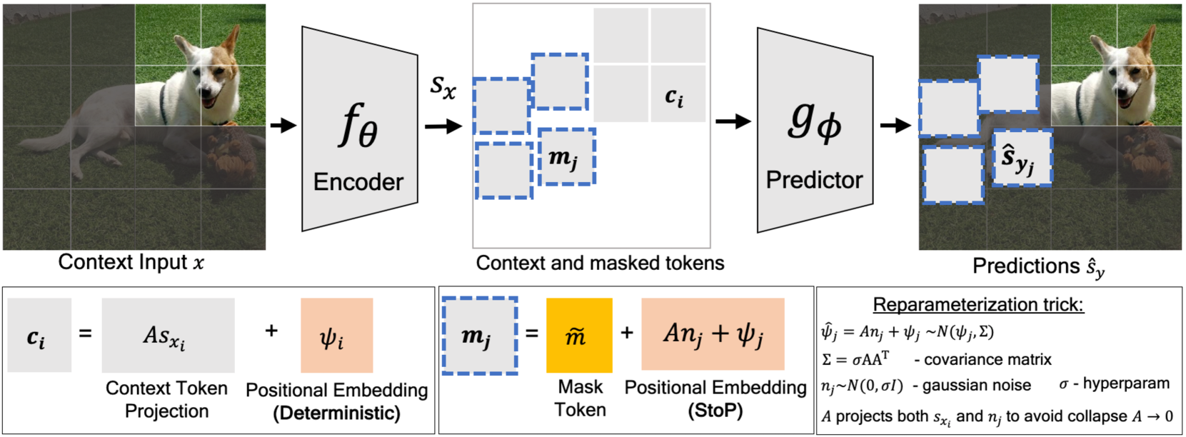
Figure 2: Masked image modeling using stochastic positional embeddings (StoP).g ϕ subscript 𝑔 italic-ϕ g_{\phi}italic_g start_POSTSUBSCRIPT italic_ϕ end_POSTSUBSCRIPT predicts target tokens given masked tokens with stochastic positions m j subscript 𝑚 𝑗 m_{j}italic_m start_POSTSUBSCRIPT italic_j end_POSTSUBSCRIPT and context tokens c i subscript 𝑐 𝑖 c_{i}italic_c start_POSTSUBSCRIPT italic_i end_POSTSUBSCRIPT obtained via f θ subscript 𝑓 𝜃 f_{\theta}italic_f start_POSTSUBSCRIPT italic_θ end_POSTSUBSCRIPT. StoP is applied to masked tokens only, leading to features that are more robust to location uncertainties.

3 Masked Image Modeling with StoP

This section presents the StoP formulation, and how to utilize it in MIM while avoiding collapsing back to deterministic positional embeddings. A high-level schematic view of the model is included in Figure2, and a pseudo-code implementation is included in Algorithm 1.

Stochastic Positional Embeddings (StoP). Instead of training the model to make predictions in exact locations, we propose to use stochastic positional embeddings which implicitly force the model to make stochastic predictions. This is meant to teach the model that locations cannot be predicted precisely, resulting in improved robustness.

Formulating StoP requires defining the distribution of the stochastic positions, parameterizing it appropriately, and implementing measures to prevent the model from scaling down the noise to the point where it becomes negligible.

Given a position j 𝑗 j italic_j, we denote by ψ^j subscript^𝜓 𝑗\hat{\psi}{j}over^ start_ARG italic_ψ end_ARG start_POSTSUBSCRIPT italic_j end_POSTSUBSCRIPT the random variable providing the position embedding. We assume that ψ^j subscript^𝜓 𝑗\hat{\psi}{j}over^ start_ARG italic_ψ end_ARG start_POSTSUBSCRIPT italic_j end_POSTSUBSCRIPT is distributed as Gaussian whose mean is the fixed embedding ψ j subscript 𝜓 𝑗\psi_{j}italic_ψ start_POSTSUBSCRIPT italic_j end_POSTSUBSCRIPT, and whose covariance matrix is Σ∈ℝ d p×d p Σ superscript ℝ subscript 𝑑 𝑝 subscript 𝑑 𝑝\Sigma\in\mathbb{R}^{d_{p}\times d_{p}}roman_Σ ∈ blackboard_R start_POSTSUPERSCRIPT italic_d start_POSTSUBSCRIPT italic_p end_POSTSUBSCRIPT × italic_d start_POSTSUBSCRIPT italic_p end_POSTSUBSCRIPT end_POSTSUPERSCRIPT:

ψ^j∼N⁢(ψ j,Σ)similar-to subscript^𝜓 𝑗 𝑁 subscript 𝜓 𝑗 Σ\hat{\psi}{j}\sim N(\psi{j},\Sigma)over^ start_ARG italic_ψ end_ARG start_POSTSUBSCRIPT italic_j end_POSTSUBSCRIPT ∼ italic_N ( italic_ψ start_POSTSUBSCRIPT italic_j end_POSTSUBSCRIPT , roman_Σ )(3)

Naturally, we want to learn an optimal Σ Σ\Sigma roman_Σ. To parameterize Σ Σ\Sigma roman_Σ, we use a general formulation of a low-rank covariance matrix:

Σ=σ⁢A⁢A T Σ 𝜎 𝐴 superscript 𝐴 𝑇\Sigma=\sigma AA^{T}roman_Σ = italic_σ italic_A italic_A start_POSTSUPERSCRIPT italic_T end_POSTSUPERSCRIPT(4)

Where A∈ℝ d p×d e 𝐴 superscript ℝ subscript 𝑑 𝑝 subscript 𝑑 𝑒 A\in\mathbb{R}^{d_{p}\times d_{e}}italic_A ∈ blackboard_R start_POSTSUPERSCRIPT italic_d start_POSTSUBSCRIPT italic_p end_POSTSUBSCRIPT × italic_d start_POSTSUBSCRIPT italic_e end_POSTSUBSCRIPT end_POSTSUPERSCRIPT is a learned matrix and σ∈ℝ+𝜎 superscript ℝ\sigma\in\mathbb{R^{+}}italic_σ ∈ blackboard_R start_POSTSUPERSCRIPT + end_POSTSUPERSCRIPT is a positive scalar hyperparameter used to control the Noise to Signal Ratio (NSR).2 2 2 At this point, it may seem unnecessary to have an additional σ 𝜎\sigma italic_σ parameter. However, later we will tie A 𝐴 A italic_A to other model parameters, and thus σ 𝜎\sigma italic_σ will not be redundant and determine the scale of the noise. By learning the matrix A 𝐴 A italic_A, this formulation allows assigning different noise levels to different location components (e.g., high and low resolution), as well as capturing correlations between location features.

Using this formulation is challenging for two reasons. First, the sampling process of ψ^^𝜓\hat{\psi}over^ start_ARG italic_ψ end_ARG is non-differential w.r.t A 𝐴 A italic_A, and therefore we cannot derive gradients to directly optimize it with SGD. Second, learning might result in the optimization process setting the values of Σ Σ\Sigma roman_Σ to zero, leading to no randomness. Next, we move to solve these issues.

Reparametrization Trick. Since ψ^j subscript^𝜓 𝑗\hat{\psi}{j}over^ start_ARG italic_ψ end_ARG start_POSTSUBSCRIPT italic_j end_POSTSUBSCRIPT is sampled from a parameterized distribution, it is non-differentiable in A 𝐴 A italic_A. However, a standard trick in these cases is to reparameterize the distribution so that the sampling is from a fixed distribution that does not depend on A 𝐴 A italic_A (e.g., see Kingma & Welling (2013)). Specifically, we generate samples from ψ^j subscript^𝜓 𝑗\hat{\psi}{j}over^ start_ARG italic_ψ end_ARG start_POSTSUBSCRIPT italic_j end_POSTSUBSCRIPT by first sampling a vector n j∈ℝ d e subscript 𝑛 𝑗 superscript ℝ subscript 𝑑 𝑒 n_{j}\in\mathbb{R}^{d_{e}}italic_n start_POSTSUBSCRIPT italic_j end_POSTSUBSCRIPT ∈ blackboard_R start_POSTSUPERSCRIPT italic_d start_POSTSUBSCRIPT italic_e end_POSTSUBSCRIPT end_POSTSUPERSCRIPT from a standard Gaussian distribution: n j∼N⁢(0,σ⁢I)similar-to subscript 𝑛 𝑗 𝑁 0 𝜎 𝐼 n_{j}\sim N(0,\sigma I)italic_n start_POSTSUBSCRIPT italic_j end_POSTSUBSCRIPT ∼ italic_N ( 0 , italic_σ italic_I ). Then, ψ^j subscript^𝜓 𝑗\hat{\psi}_{j}over^ start_ARG italic_ψ end_ARG start_POSTSUBSCRIPT italic_j end_POSTSUBSCRIPT is set to:

ψ^j=A⁢n j+ψ j subscript^𝜓 𝑗 𝐴 subscript 𝑛 𝑗 subscript 𝜓 𝑗\hat{\psi}{j}=An{j}+\psi_{j}\vspace{-5pt}over^ start_ARG italic_ψ end_ARG start_POSTSUBSCRIPT italic_j end_POSTSUBSCRIPT = italic_A italic_n start_POSTSUBSCRIPT italic_j end_POSTSUBSCRIPT + italic_ψ start_POSTSUBSCRIPT italic_j end_POSTSUBSCRIPT(5)

The resulting distribution of ψ^j subscript^𝜓 𝑗\hat{\psi}_{j}over^ start_ARG italic_ψ end_ARG start_POSTSUBSCRIPT italic_j end_POSTSUBSCRIPT is equal to that in Equation3, however, we can now differentiate directly through A 𝐴 A italic_A.

Collapse to deterministic positions (A=0). Intuitively, adding noise to an objective hurts the training loss, and thus if A 𝐴 A italic_A appears only in (5), training should set it to zero. We indeed observe this empirically, suggesting that A 𝐴 A italic_A cannot only appear in a single place in the model. In what follows we propose an approach to overcoming this issue.

Algorithm 1 MIM w/ StoP pseudo-code. requires only a minor implementation change, highlighted in light gray.

1:Input: num iterations

K 𝐾 K italic_K , image dist

S 𝑆 S italic_S , hyperparam

σ 𝜎\sigma italic_σ , positional embeddings

ψ 𝜓\psi italic_ψ

2:Params:

A,m𝐴𝑚{A,\tilde{m}}italic_A , over~ start_ARG italic_m end_ARG , encoder

f θ subscript 𝑓 𝜃 f_{\theta}italic_f start_POSTSUBSCRIPT italic_θ end_POSTSUBSCRIPT , predictor

g ϕ subscript 𝑔 italic-ϕ g_{\phi}italic_g start_POSTSUBSCRIPT italic_ϕ end_POSTSUBSCRIPT

3:for

i⁢t⁢r=1,2,…,K 𝑖 𝑡 𝑟 1 2…𝐾 itr=1,2,...,K italic_i italic_t italic_r = 1 , 2 , … , italic_K do

4:

I x∼S similar-to subscript 𝐼 𝑥 𝑆 I_{x}\sim S italic_I start_POSTSUBSCRIPT italic_x end_POSTSUBSCRIPT ∼ italic_S

5:

p←patchify⁢(I x)←𝑝 patchify subscript 𝐼 𝑥 p\leftarrow\text{patchify}(I_{x})italic_p ← patchify ( italic_I start_POSTSUBSCRIPT italic_x end_POSTSUBSCRIPT )

6:

(x,B x),(y,B y)←mask⁢(p)←𝑥 subscript 𝐵 𝑥 𝑦 subscript 𝐵 𝑦 mask 𝑝(x,B_{x}),(y,B_{y})\leftarrow\text{mask}(p)( italic_x , italic_B start_POSTSUBSCRIPT italic_x end_POSTSUBSCRIPT ) , ( italic_y , italic_B start_POSTSUBSCRIPT italic_y end_POSTSUBSCRIPT ) ← mask ( italic_p )

7:

s x←f θ⁢(x)←subscript 𝑠 𝑥 subscript 𝑓 𝜃 𝑥 s_{x}\leftarrow f_{\theta}(x)italic_s start_POSTSUBSCRIPT italic_x end_POSTSUBSCRIPT ← italic_f start_POSTSUBSCRIPT italic_θ end_POSTSUBSCRIPT ( italic_x )

8:# apply StoP on a sequence of tokens

9:n j∼𝒩(0,σ I n_{j}\sim\mathcal{N}(0,\sigma I italic_n start_POSTSUBSCRIPT italic_j end_POSTSUBSCRIPT ∼ caligraphic_N ( 0 , italic_σ italic_I)

10:# ψ B x subscript 𝜓 subscript 𝐵 𝑥\psi_{B_{x}}italic_ψ start_POSTSUBSCRIPT italic_B start_POSTSUBSCRIPT italic_x end_POSTSUBSCRIPT end_POSTSUBSCRIPT, ψ B y subscript 𝜓 subscript 𝐵 𝑦\psi_{B_{y}}italic_ψ start_POSTSUBSCRIPT italic_B start_POSTSUBSCRIPT italic_y end_POSTSUBSCRIPT end_POSTSUBSCRIPT - masked/context positional embeddings

11:

m=𝑚 absent m=italic_m = A⁢n 𝐴 𝑛 An italic_A italic_n

+ψ B y+msubscript 𝜓 subscript 𝐵 𝑦𝑚+\psi_{B_{y}}+\tilde{m}+ italic_ψ start_POSTSUBSCRIPT italic_B start_POSTSUBSCRIPT italic_y end_POSTSUBSCRIPT end_POSTSUBSCRIPT + over~ start_ARG italic_m end_ARG

12:

c=A⁢s x+ψ B x 𝑐 𝐴 subscript 𝑠 𝑥 subscript 𝜓 subscript 𝐵 𝑥 c=As_{x}+\psi_{B_{x}}italic_c = italic_A italic_s start_POSTSUBSCRIPT italic_x end_POSTSUBSCRIPT + italic_ψ start_POSTSUBSCRIPT italic_B start_POSTSUBSCRIPT italic_x end_POSTSUBSCRIPT end_POSTSUBSCRIPT

13:# predict targets

14:

s^y←g ϕ⁢(c,m)←subscript^𝑠 𝑦 subscript 𝑔 italic-ϕ 𝑐 𝑚\hat{s}{y}\leftarrow g{\phi}(c,m)over^ start_ARG italic_s end_ARG start_POSTSUBSCRIPT italic_y end_POSTSUBSCRIPT ← italic_g start_POSTSUBSCRIPT italic_ϕ end_POSTSUBSCRIPT ( italic_c , italic_m )

15:

s y←get_target⁢(y)←subscript 𝑠 𝑦 get_target 𝑦 s_{y}\leftarrow\text{get_target}(y)italic_s start_POSTSUBSCRIPT italic_y end_POSTSUBSCRIPT ← get_target ( italic_y )

16:

loss←L⁢(s^y,s y)←loss 𝐿 subscript^𝑠 𝑦 subscript 𝑠 𝑦\text{loss}\leftarrow L(\hat{s}{y},s{y})loss ← italic_L ( over^ start_ARG italic_s end_ARG start_POSTSUBSCRIPT italic_y end_POSTSUBSCRIPT , italic_s start_POSTSUBSCRIPT italic_y end_POSTSUBSCRIPT )

17:

sgd_step⁢(loss;{θ,ϕ,A,m})sgd_step loss 𝜃 italic-ϕ 𝐴𝑚\text{sgd_step}(\text{loss};{\theta,\phi,A,\tilde{m}})sgd_step ( loss ; { italic_θ , italic_ϕ , italic_A , over~ start_ARG italic_m end_ARG } )

18:end for

Avoiding collapse by weight tying A=B. To avoid the collapse to deterministic positions, we propose to tie the weights of A 𝐴 A italic_A and B 𝐵 B italic_B (originally defined in Eq.1), such that the same matrix A 𝐴 A italic_A projects both the context tokens s x i subscript 𝑠 subscript 𝑥 𝑖 s_{x_{i}}italic_s start_POSTSUBSCRIPT italic_x start_POSTSUBSCRIPT italic_i end_POSTSUBSCRIPT end_POSTSUBSCRIPT and the noise tokens n j subscript 𝑛 𝑗 n_{j}italic_n start_POSTSUBSCRIPT italic_j end_POSTSUBSCRIPT:

c i=A⁢s x i+ψ i m j=A⁢n j+ψ j+mformulae-sequence subscript 𝑐 𝑖 𝐴 subscript 𝑠 subscript 𝑥 𝑖 subscript 𝜓 𝑖 subscript 𝑚 𝑗 𝐴 subscript 𝑛 𝑗 subscript 𝜓 𝑗𝑚 c_{i}=As_{x_{i}}+\psi_{i}\quad m_{j}=An_{j}+\psi_{j}+\tilde{m}italic_c start_POSTSUBSCRIPT italic_i end_POSTSUBSCRIPT = italic_A italic_s start_POSTSUBSCRIPT italic_x start_POSTSUBSCRIPT italic_i end_POSTSUBSCRIPT end_POSTSUBSCRIPT + italic_ψ start_POSTSUBSCRIPT italic_i end_POSTSUBSCRIPT italic_m start_POSTSUBSCRIPT italic_j end_POSTSUBSCRIPT = italic_A italic_n start_POSTSUBSCRIPT italic_j end_POSTSUBSCRIPT + italic_ψ start_POSTSUBSCRIPT italic_j end_POSTSUBSCRIPT + over~ start_ARG italic_m end_ARG(6)

This tying means that the scale of the noise and the input are both determined by A 𝐴 A italic_A, and thus the noise cannot be set to zero, without affecting other parts of the model. This can be understood by considering two extreme cases:

• •If A=0 𝐴 0 A=0 italic_A = 0, there is complete certainty about the positional embeddings but all context is lost (A⁢s x i=0 𝐴 subscript 𝑠 subscript 𝑥 𝑖 0 As_{x_{i}}=0 italic_A italic_s start_POSTSUBSCRIPT italic_x start_POSTSUBSCRIPT italic_i end_POSTSUBSCRIPT end_POSTSUBSCRIPT = 0).
• •If A 𝐴 A italic_A has large magnitude, the context information is preserved but the noise is amplified and camouflages masked tokens positional embeddings (A⁢n j≫ψ j much-greater-than 𝐴 subscript 𝑛 𝑗 subscript 𝜓 𝑗 An_{j}\gg\psi_{j}italic_A italic_n start_POSTSUBSCRIPT italic_j end_POSTSUBSCRIPT ≫ italic_ψ start_POSTSUBSCRIPT italic_j end_POSTSUBSCRIPT).

This dual role of A 𝐴 A italic_A forces the model to trade-off between the positions of the masked tokens and the context tokens.3 3 3 Note that an implicit assumption here is that ψ 𝜓\psi italic_ψ and s x subscript 𝑠 𝑥 s_{x}italic_s start_POSTSUBSCRIPT italic_x end_POSTSUBSCRIPT have fixed magnitude. This is true for sine-cosine features and for s x subscript 𝑠 𝑥 s_{x}italic_s start_POSTSUBSCRIPT italic_x end_POSTSUBSCRIPT which are layer normalized by the transformer last layer.

In the following proposition, we formally show that if the weights A 𝐴 A italic_A and B 𝐵 B italic_B are tied then A 𝐴 A italic_A cannot collapse. More specifically, A=0 𝐴 0 A=0 italic_A = 0 occurs only if in the original deterministic setting B 𝐵 B italic_B goes to zero and doesn’t utilize the context anyway. Formally, consider a regression task where F 𝐹 F italic_F predicts some target y j subscript 𝑦 𝑗 y_{j}italic_y start_POSTSUBSCRIPT italic_j end_POSTSUBSCRIPT given a stochastic position A⁢n j+ψ j+m𝐴 subscript 𝑛 𝑗 subscript 𝜓 𝑗𝑚 An_{j}+\psi_{j}+\tilde{m}italic_A italic_n start_POSTSUBSCRIPT italic_j end_POSTSUBSCRIPT + italic_ψ start_POSTSUBSCRIPT italic_j end_POSTSUBSCRIPT + over~ start_ARG italic_m end_ARG where n j∼N⁢(0,σ⁢I)similar-to subscript 𝑛 𝑗 𝑁 0 𝜎 𝐼 n_{j}\sim N(0,\sigma I)italic_n start_POSTSUBSCRIPT italic_j end_POSTSUBSCRIPT ∼ italic_N ( 0 , italic_σ italic_I ) and projected context token B⁢x i 𝐵 subscript 𝑥 𝑖 Bx_{i}italic_B italic_x start_POSTSUBSCRIPT italic_i end_POSTSUBSCRIPT. Denote J t⁢i⁢e⁢d,J d⁢e⁢t subscript 𝐽 𝑡 𝑖 𝑒 𝑑 subscript 𝐽 𝑑 𝑒 𝑡 J_{tied},J_{det}italic_J start_POSTSUBSCRIPT italic_t italic_i italic_e italic_d end_POSTSUBSCRIPT , italic_J start_POSTSUBSCRIPT italic_d italic_e italic_t end_POSTSUBSCRIPT the loss functions when tying the weights A 𝐴 A italic_A and B 𝐵 B italic_B, and when using deterministic positional embeddings respectively:

J t⁢i⁢e⁢d⁢(A)=∑i,j 𝔼 n j⁢[(F⁢(A⁢n j+ψ j+m,A⁢x i)−y j)2]subscript 𝐽 𝑡 𝑖 𝑒 𝑑 𝐴 subscript 𝑖 𝑗 subscript 𝔼 subscript 𝑛 𝑗 delimited-[]superscript 𝐹 𝐴 subscript 𝑛 𝑗 subscript 𝜓 𝑗𝑚 𝐴 subscript 𝑥 𝑖 subscript 𝑦 𝑗 2 J_{tied}(A)=\sum_{i,j}\mathbb{E}{n{j}}[(F(An_{j}+\psi_{j}+\tilde{m},Ax_{i})-% y_{j})^{2}]italic_J start_POSTSUBSCRIPT italic_t italic_i italic_e italic_d end_POSTSUBSCRIPT ( italic_A ) = ∑ start_POSTSUBSCRIPT italic_i , italic_j end_POSTSUBSCRIPT blackboard_E start_POSTSUBSCRIPT italic_n start_POSTSUBSCRIPT italic_j end_POSTSUBSCRIPT end_POSTSUBSCRIPT [ ( italic_F ( italic_A italic_n start_POSTSUBSCRIPT italic_j end_POSTSUBSCRIPT + italic_ψ start_POSTSUBSCRIPT italic_j end_POSTSUBSCRIPT + over~ start_ARG italic_m end_ARG , italic_A italic_x start_POSTSUBSCRIPT italic_i end_POSTSUBSCRIPT ) - italic_y start_POSTSUBSCRIPT italic_j end_POSTSUBSCRIPT ) start_POSTSUPERSCRIPT 2 end_POSTSUPERSCRIPT ]

J d⁢e⁢t⁢(B)=∑i,j[(F⁢(ψ j+m,B⁢x i)−y j)2]subscript 𝐽 𝑑 𝑒 𝑡 𝐵 subscript 𝑖 𝑗 delimited-[]superscript 𝐹 subscript 𝜓 𝑗𝑚 𝐵 subscript 𝑥 𝑖 subscript 𝑦 𝑗 2 J_{det}(B)=\sum_{i,j}[(F(\psi_{j}+\tilde{m},Bx_{i})-y_{j})^{2}]italic_J start_POSTSUBSCRIPT italic_d italic_e italic_t end_POSTSUBSCRIPT ( italic_B ) = ∑ start_POSTSUBSCRIPT italic_i , italic_j end_POSTSUBSCRIPT [ ( italic_F ( italic_ψ start_POSTSUBSCRIPT italic_j end_POSTSUBSCRIPT + over~ start_ARG italic_m end_ARG , italic_B italic_x start_POSTSUBSCRIPT italic_i end_POSTSUBSCRIPT ) - italic_y start_POSTSUBSCRIPT italic_j end_POSTSUBSCRIPT ) start_POSTSUPERSCRIPT 2 end_POSTSUPERSCRIPT ]

Proposition 3.1.

If the weights of A 𝐴 A italic_A and B 𝐵 B italic_B are tied (namely A=B 𝐴 𝐵 A=B italic_A = italic_B) then d⁢J t⁢i⁢e⁢d d⁢A|A=0=0 evaluated-at 𝑑 subscript 𝐽 𝑡 𝑖 𝑒 𝑑 𝑑 𝐴 𝐴 0 0\left.\frac{dJ_{tied}}{dA}\right|{A=0}=0 divide start_ARG italic_d italic_J start_POSTSUBSCRIPT italic_t italic_i italic_e italic_d end_POSTSUBSCRIPT end_ARG start_ARG italic_d italic_A end_ARG | start_POSTSUBSCRIPT italic_A = 0 end_POSTSUBSCRIPT = 0 iff d⁢J d⁢e⁢t d⁢B|B=0=0 evaluated-at 𝑑 subscript 𝐽 𝑑 𝑒 𝑡 𝑑 𝐵 𝐵 0 0\left.\frac{dJ{det}}{dB}\right|_{B=0}=0 divide start_ARG italic_d italic_J start_POSTSUBSCRIPT italic_d italic_e italic_t end_POSTSUBSCRIPT end_ARG start_ARG italic_d italic_B end_ARG | start_POSTSUBSCRIPT italic_B = 0 end_POSTSUBSCRIPT = 0

Proof is included in AppendixA.

Optimal Predictor. Our approach relies on using stochastic positional embeddings. Here we provide further analysis, showing that the optimal predictor performs spatial smoothing. Consider a random variable X 𝑋 X italic_X (corresponding to the context in our case. For simplicity assume X 𝑋 X italic_X is just the positional embedding of the context) that is used to predict a variable Y 𝑌 Y italic_Y (corresponding to the target in our case). But now instead of predicting from X 𝑋 X italic_X, we use a noise variable Z 𝑍 Z italic_Z that is independent of both X,Y 𝑋 𝑌 X,Y italic_X , italic_Y, and provide the predictor with only the noisy result R=g⁢(X,Z)𝑅 𝑔 𝑋 𝑍 R=g(X,Z)italic_R = italic_g ( italic_X , italic_Z ). Here g 𝑔 g italic_g is some mixing function (in our case g⁢(x,z)=x+z 𝑔 𝑥 𝑧 𝑥 𝑧 g(x,z)=x+z italic_g ( italic_x , italic_z ) = italic_x + italic_z). We next derive the optimal predictor f⁢(R)𝑓 𝑅 f(R)italic_f ( italic_R ) in this case. Formally we want to minimize:

E R,Y⁢[(f⁢(R)−Y)2]subscript 𝐸 𝑅 𝑌 delimited-[]superscript 𝑓 𝑅 𝑌 2 E_{R,Y}[(f(R)-Y)^{2}]italic_E start_POSTSUBSCRIPT italic_R , italic_Y end_POSTSUBSCRIPT ( italic_f ( italic_R ) - italic_Y ) start_POSTSUPERSCRIPT 2 end_POSTSUPERSCRIPT

Proposition 3.2.

If Z 𝑍 Z italic_Z is a Gaussian with zero mean and unit variance, the optimal predictor that minimizes Equation7 is:

f⁢(r)=∫x E⁢[Y|X=x]⁢1 2⁢π⁢e−0.5⁢(x−r)2⁢𝑑 x 𝑓 𝑟 subscript 𝑥 𝐸 delimited-[]conditional 𝑌 𝑋 𝑥 1 2 𝜋 superscript 𝑒 0.5 superscript 𝑥 𝑟 2 differential-d 𝑥 f(r)=\int_{x}E[Y|X=x]\frac{1}{\sqrt{2\pi}}e^{-0.5(x-r)^{2}}dx italic_f ( italic_r ) = ∫ start_POSTSUBSCRIPT italic_x end_POSTSUBSCRIPT italic_E [ italic_Y | italic_X = italic_x ] divide start_ARG 1 end_ARG start_ARG square-root start_ARG 2 italic_π end_ARG end_ARG italic_e start_POSTSUPERSCRIPT - 0.5 ( italic_x - italic_r ) start_POSTSUPERSCRIPT 2 end_POSTSUPERSCRIPT end_POSTSUPERSCRIPT italic_d italic_x

Thus, the optimal predictor amounts to a convolution of the clean expected values with a Gaussian. See AppendixB for the proof.

4 Experiments and Results

Next, we turn to discuss the main experiments presented in the paper. In Section4.1, we describe the application of StoP to various downstream tasks including image recognition, dense prediction, and low-level vision tasks. In Section4.2 we discuss the ablation study and design choices. The full implementation details are included in AppendixC.

4.1 Downstream Tasks

We conducted pre-training of StoP on top of I-JEPA, which is a state-of-the-art MIM model. We train on IN-1k for a period of 600 600 600 600 epochs using ViT-B/16 and ViT-L/16 architectures for the encoder and predictor or for 300 300 300 300 epochs when using ViT-H/14. Subsequently, we proceeded to evaluate the model’s performance on a variety of downstream tasks. Additional results and comparison to invariance-based approaches are included AppendixC.2.

Table 1: StoP compared to deterministic sinusoidal positional embeddings on IN-1k. StoP leads to consistent linear probing improvement in all settings. When applying linear probing on a trained ViT-H model with StoP, using only 1%percent 1 1%1 % of the labeled data and using averaged pooled features from the last layer, StoP results in an +2.5% improvement. The baseline I-JEPA uses sinusoidal positional embeddings.

Image recognition. For image classification, we perform a linear probing evaluation of StoP on multiple datasets, including ImageNet (IN-1k)(Russakovsky et al., 2015), Places 205(Zhou et al., 2014a), iNaturalist 2018(Van Horn et al., 2018), and CIFAR 100(Krizhevsky, 2009). These datasets vary in their size, their purpose, and the geographical environments from which the images were captured. For example, IN-1k contains over 1.2 1.2 1.2 1.2 million images compared to CIFAR-100 which contains only 60,000 60 000 60,000 60 , 000 images, and while IN-1k is focused on object recognition, iNaturalist and Places are focused on scene and species recognition.

Table 2: Linear-evaluation on IN-1k. Replacing sinusoidal positional embeddings with StoP in I-JEPA significantly improves linear probing results.

Table 3: Video objects semi-supervised segmentation. MIM with StoP learns features with a finer level of granularity. Results are reported on DAVIS 2017 dataset.

In Table1, we present the linear probing image classification results conducted on IN-1k under different linear evaluation protocols using different amounts of data, and by aggregating features from different layers. E.g, “100%, last 4 layers” applies linear probing on the entire IN-1k data and the representation of each image is comprised of a concatenation of four feature vectors, each one summarizes information from its corresponding layer via average pooling. In Table2 we compare linear probing results of common MIM methods on IN-1k, reporting past published performance. In Table2 all perform linear probing over the output from the last layer.

StoP improves the baseline performance using all architectures examined. For example, +2.5%percent 2.5+2.5%+ 2.5 % linear probing performance gains with ViT-H using 1%percent 1 1%1 % of the labeled data and 1.6%percent 1.6 1.6%1.6 % when using features from the last 4 4 4 4 layers using ViT-B on the full IN-1k data. Furthermore, using StoP leads to improvements in downstream linear probing tasks (see Table4). For example, StoP leads to 3.3%percent 3.3 3.3%3.3 % improvement on iNAT using ViT-H and 1.3% on counting. This confirms that the learned representations lead to improvements in a large variety of image recognition tasks. On full finetuning using 1% of the labeled data, we observe similar performance improvements (see Table5), e.g, +2.3%percent 2.3+2.3%+ 2.3 % improvements on Top-1 accuracy using ViT-L model. We provide the full finetuning results in Table16, AppendixC.2.

Table 4: Linear-probe transfer for various downstream tasks. Linear-evaluation on downstream image classification, object counting, and depth ordering tasks. Using StoP instead of sinusoidal deterministic positions leads to improvements on all tasks. E.g, +3.3%percent 3.3+3.3%+ 3.3 % on iNAT18 and +1.3%percent 1.3+1.3%+ 1.3 % on Counting.

Counting and depth ordering. We assess the downstream performance on tasks that require fine-grained objects representations like counting and depth ordering using the CLEVR(Johnson et al., 2017) dataset. Table4 provides evidence that using StoP significantly improve counting (+1.3%percent 1.3+1.3%+ 1.3 %) and slightly improve depth ordering (+0.1%percent 0.1+0.1%+ 0.1 %).

Dense prediction. To evaluate how well StoP performs on dense prediction tasks, e.g, tasks that require fine-grained spatial representations, we utilized the learned models for semi-supervised video object segmentation on the DAVIS 2017(Pont-Tuset et al., 2017) dataset. We follow previous works (e.g Jabri et al. (2020); Caron et al. (2021)) and use the pretrained model to extract frames features and use patch-level affinities between frames to track the first segmentation mask. We include video semi-supervised video-object segmentation by tracking results in Table3. We find that StoP significantly improves over I-JEPA with deterministic sinusoidal location features. For example, we observe an improvement of +2.5%percent 2.5+2.5%+ 2.5 % in J&F 𝐽 𝐹 J&F italic_J & italic_F using ViT-L.

4.2 Ablation Study

Table 5: Finetuning results over IN-1k with 1% labels. StoP significantly improves finetuning performance compared to using sine-cosine positional embeddings. Using ViT-L/16 architecture.

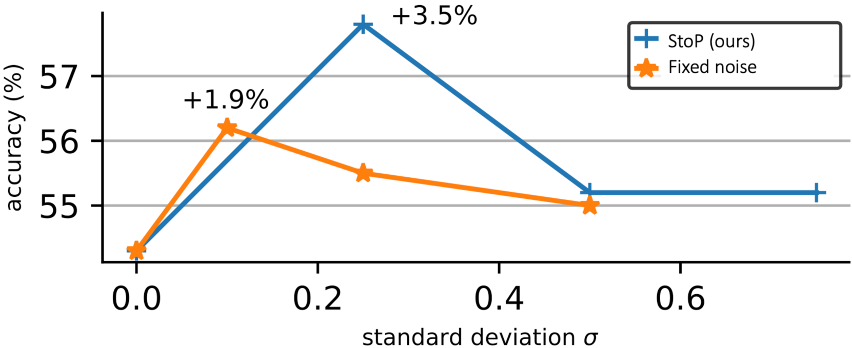
Figure 3: Learned vs. predefined stochastic positions. Using the learned covariance matrix as in StoP, e.g, Σ=σ⁢A⁢A T normal-Σ 𝜎 𝐴 superscript 𝐴 𝑇\Sigma=\sigma AA^{T}roman_Σ = italic_σ italic_A italic_A start_POSTSUPERSCRIPT italic_T end_POSTSUPERSCRIPT leads to +3.5%percent 3.5+3.5%+ 3.5 % improvement compared to smaller gains with a fixed covariance matrix Σ=σ⁢I normal-Σ 𝜎 𝐼\Sigma=\sigma I roman_Σ = italic_σ italic_I. Accuracy is reported based on linear probing evaluation using 1% of the data from IN-1k.

Table 6: Different positional embeddings. Linear probing on IN-1K using only 1% of the labels. Stochastic Positions (StoP) outperforms other common deterministic variants by 3.3%percent 3.3 3.3%3.3 %.

Our primary focus is to evaluate the effectiveness of StoP. To demonstrate this, we assess various design options using ViT-B architecture for the encoder and predictor. We pre-train for 300 300 300 300 epochs on IN-1k based on the I-JEPA(Assran et al., 2023) MIM model. We then assessed the linear probing performance on IN-1k using only 1% of the labels.

StoP compared to deterministic positional embeddings. The most common choices for positional embeddings for Vision Transformers are sine-cosine location features (also used in MAE, I-JEPA) and learned positional embedding. We evaluate the MIM downstream performance using each of these options and using StoP (see Table6). The results indicate that using StoP improves the performance by +3.2%percent 3.2+3.2%+ 3.2 % compared to sinusoidal and learned positional embeddings.

Learned vs. predefined covariance matrix. To confirm that learning the covariance matrix Σ=σ⁢A⁢A T Σ 𝜎 𝐴 superscript 𝐴 𝑇\Sigma=\sigma AA^{T}roman_Σ = italic_σ italic_A italic_A start_POSTSUPERSCRIPT italic_T end_POSTSUPERSCRIPT (and specifically A 𝐴 A italic_A) is beneficial compared to using a predefined covariance matrix, we compare to stochastic positional embeddings with a predefined covariance matrix Σ=σ⁢I Σ 𝜎 𝐼\Sigma=\sigma I roman_Σ = italic_σ italic_I, without any learning. We compare both options using different σ 𝜎\sigma italic_σ hyperparameter values. Figure3 indicates that it is advantageous to learn Σ Σ\Sigma roman_Σ rather than use fixed parameters. Our findings show that setting the hyperparameter value to σ=0.25 𝜎 0.25\sigma=0.25 italic_σ = 0.25 leads to an improvement of 3.5%percent 3.5 3.5%3.5 % points compared to deterministic positional embeddings (σ=0 𝜎 0\sigma=0 italic_σ = 0).

Application of StoP to different tokens. We apply StoP to context and/or masked tokens. The results in Table7 confirm our design choice, showing that StoP is most beneficial when it is applied solely to masked tokens, compared to context tokens, or both masked and context tokens.

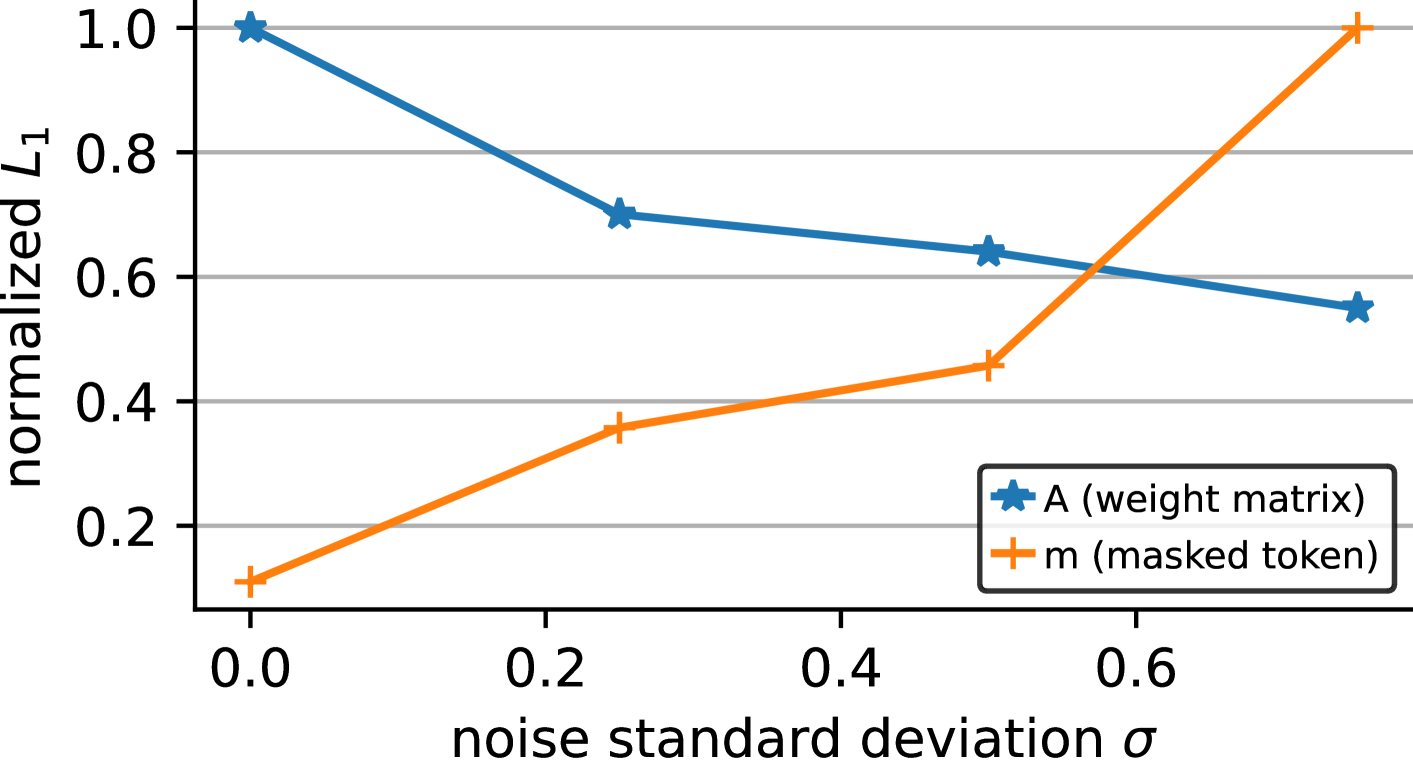
Figure 4: Increasing σ 𝜎\sigma italic_σ induces regularization. Changing the prior σ 𝜎\sigma italic_σ (where Σ=σ⁢A⁢A T normal-Σ 𝜎 𝐴 superscript 𝐴 𝑇\Sigma=\sigma AA^{T}roman_Σ = italic_σ italic_A italic_A start_POSTSUPERSCRIPT italic_T end_POSTSUPERSCRIPT) induces regularization over A 𝐴 A italic_A and increases the norm of the masked token, which preserves the masked token information in comparison to the added noise.

Table 7: Applying noise to different tokens. Applying learned noise to context and/or masked tokens positional embeddings (sine-cosine). Reporting linear evaluation accuracy (using 1% of IN-1k).

4.3 Analysis

To explain how StoP affects MIM, we analyze the learned model weights, visualize the stochastic positional embeddings, and visualize the predicted features.

StoP induces regularization. The matrix A 𝐴 A italic_A is used to project both noise tokens and context embedding tokens. We hypothesize that StoP implicitly regularizes A 𝐴 A italic_A. To test this hypothesis we train models using StoP changing only the hyperparam σ 𝜎\sigma italic_σ (see Figure4). We find that increasing the value of σ 𝜎\sigma italic_σ leads to a decrease in the norm of A 𝐴 A italic_A, which can be viewed as regularization. On the other hand, increasing σ 𝜎\sigma italic_σ leads to an increase in the norm of the masked token bias m~~𝑚\tilde{m}over~ start_ARG italic_m end_ARG. We speculate that the masked token bias increases in scale to prevent losing its information relative to the noise.

To further analyze this phenomenon, we train additional models while applying l 1 subscript 𝑙 1 l_{1}italic_l start_POSTSUBSCRIPT 1 end_POSTSUBSCRIPT or l 2 subscript 𝑙 2 l_{2}italic_l start_POSTSUBSCRIPT 2 end_POSTSUBSCRIPT regularization on A 𝐴 A italic_A while keeping the positional embeddings of masked tokens deterministic. We find that StoP leads to +2%percent 2 2%2 % improvement over l 1 subscript 𝑙 1 l_{1}italic_l start_POSTSUBSCRIPT 1 end_POSTSUBSCRIPT and +2.1%percent 2.1 2.1%2.1 % over l 2 subscript 𝑙 2 l_{2}italic_l start_POSTSUBSCRIPT 2 end_POSTSUBSCRIPT regualrization. Therefore, we conclude that StoP is superior to simple regularization.

Stochastic positional embedding visualization.

Table 8: Low resolution prediction. Performance of StoP compared to models that predict features on lower scales via max pooling or bilinear resizing. Reporting linear evaluation accuracy (using 1% of IN-1k). StoP performs better than low res prediction.

To visualize how StoP affects the similarity between different positions, we plot the similarity matrix between a stochastic position embedding query and the predefined sine-cosine deterministic positions (Figure5). With StoP, we find that query locations are more similar to a wider range of neighboring locations. Building on this observation, we train models to investigate if directly predicting lower-scale features is beneficial. We trained models to predict features in both the original scale and a downscaled version by a factor of 2, using bilinear resizing and max pooling for downscaling. However, we found that predicting lower scale features does not improve performance (see Table8).

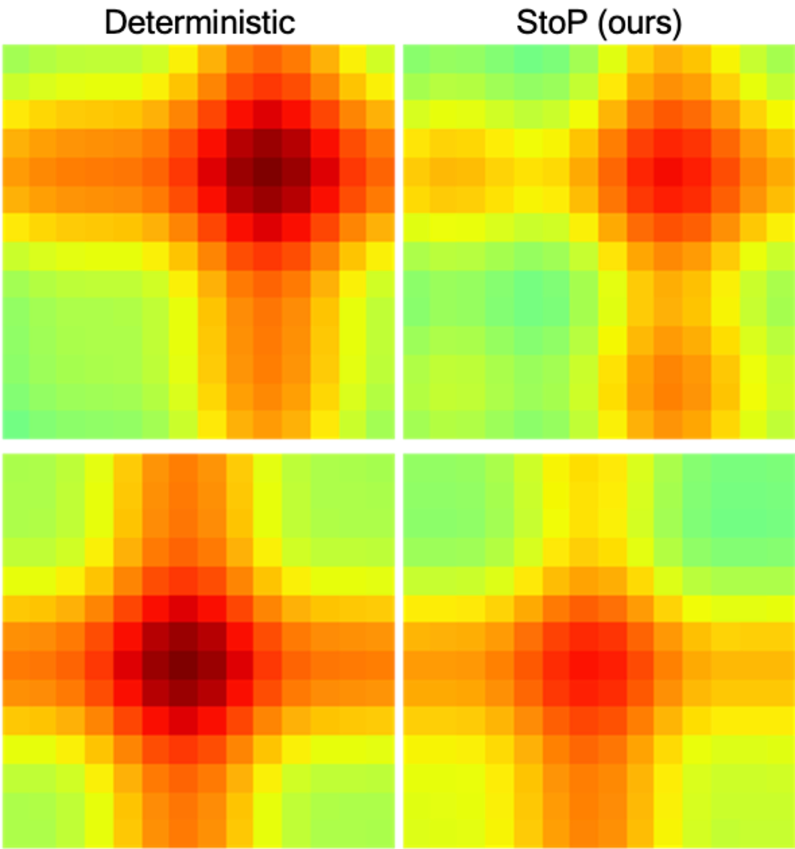
Figure 5: Similarity matrices of deterministic and stochastic positional embedding (StoP) to a query position. Each row represents the similarity given a different query position. StoP leads to a spatially smooth similarity matrix, thereby making it hard to distinguish the exact location of a given patch.

Figure 6: Feature visualization. We plot the similarity between the predicted features of a given patch (marked in white within the masked black area) and other features in the same image. Using StoP produces features that are less location based compared to I-JEPA baseline that have strong correlation with the target location.

Prediction visualization. We include heatmap visualization to visualize the similarity of a predicted token to all other tokens within the same image (see Figure6). For a given image, mask, and a masked patch of interest, we apply cosine similarity between the predicted patch and all other token representations within the same image, followed by a softmax. For I-JEPA with sine-cosine positional embeddings, the visualization indicates that adjacent tokens tend to share similar features, implying a correlation between the features and spatial location. In contrast, StoP produces predictions correlated with non-neighboring small areas. We speculate that using StoP leads to learning features that are more semantic and prevents overfitting to location features.

5 Related Work

Masked image modeling (MIM). There is a significant body of research exploring visual representation learning by predicting corrupted sensory inputs. Denoising autoencoders(Vincent et al., 2010), for example, use random noise as input corruption, while context encoders(Pathak et al., 2016) regress an entire image region based on its surrounding. The idea behind masked image modeling(He et al., 2021; Xie et al., 2021; Bao et al., 2021) has emerged as a way to address image denoising. In this approach, a Vision Transformer(Dosovitskiy et al., 2020) is used to reconstruct missing input patches. The Masked Autoencoders (MAE) architecture(He et al., 2021), for example, efficiently reconstructs missing patches in pixel space and achieves strong performance on large labeled datasets. Other approaches, such as BEiT(Bao et al., 2021), predict a latent code obtained using a pretrained tokenizer. However, pixel-level pre-training has been shown to outperform BEiT in fine-tuning. SimMiM(Xie et al., 2021) explores simple reconstruction targets like color clusters but shows no significant advantages over pixel space reconstruction. Recently, Image-JEPA (I-JEPA)(Assran et al., 2023; LeCun, 2022) was proposed as a non-generative approach for self-supervised learning of semantic image representations. I-JEPA predicts the representations of various target blocks in an image from a single context block to guide it toward producing semantic representations. Our approach builds on this line of work and we propose to deal with location uncertainty using stochastic positional embeddings which was not explored before.

Positional Embeddings in Transformers. One of the core components of the Transformer architecture(Vaswani et al., 2017) is the Self-Attention block, which is a permutation invariant function, e.g, changing the order of the input tokens does not change the function output. Consequently, it is necessary to feed input tokens together with their positional embedding to describe their location. Absolute positional embeddings like fixed 2D sinusoidal features(Bello et al., 2019) or learned location features are the prevalent type of positional embeddings for the Vision Transformer(Dosovitskiy et al., 2020). Relative positional embeddings have recently gained popularity in NLP due to their ability to address the gap between the training and testing sequence length(Su et al., 2021; Chu et al., 2021; Press et al., 2021). For example, (Press et al., 2021) proposed ALiBi to bias self-attention to assign higher confidence to neighboring locations, and SPE(Liutkus et al., 2021) proposed a stochastic approximation for relative positional embedding in linear transformers. Differently, we propose StoP to tackle location uncertainties in MIM, and it can be easily applied on top of any existing deterministic variant.

Invariance-based methods. These methods incorporate a loss that encourages similarity between augmented views of the the same image while avoiding a trivial solution. For example, contrastive learning prevents collapse by introducing negative examples(Hadsell et al., 2006; Dosovitskiy et al., 2014; Chen et al., 2020a; He et al., 2019; Chen et al., 2020b; Dwibedi et al., 2021). This can be achieved using a memory bank of previous instances (Wu et al., 2018; Oord et al., 2018; Tian et al., 2019; Misra & van der Maaten, 2020). However, there are also non-contrastive solutions that have been proposed. Of particular interest, a momentum encoder has been shown to prevent collapse even without negative pairs(Grill et al., 2020; Caron et al., 2021; Salakhutdinov & Hinton, 2007). Other methods include stopping the gradient to one branch(Chen & He, 2021) or applying regularization using batch statistics(Zbontar et al., 2021; Bardes et al., 2021, 2022; Ermolov et al., 2020; Hua et al., 2021). MoCo v3(Chen et al., 2021), then DINO(Caron et al., 2021) extended these approaches for Vision Transformer, and iBOT(Zhou et al., 2021) proposed to add a MIM loss to DINO. These approaches perform extremely well on ImageNet linear-probing, yet they rely on batch statistics, struggle under non-uniform distributions(Assran et al., 2022), and require hand-crafted image augmentations(Xiao et al.,). Our approach is based on MIM that requires less assumptions on batch statistics or handcrafted invariances.

6 Limitations

We applied StoP to I-JEPA which performs image reconstruction in the feature space. However, our attempts to apply StoP to MIM that use pixel based reconstruction, mainly MAE, were not successful. We speculate that adding StoP to MAE might make pixel reconstruction too difficult to achieve. Additionally, StoP tackles location uncertainty but not appearance uncertainty, which we believe is implicitly modeled by reconstructing tokens in feature space. Also, when modeling stochastic positions it may might be possible to condition the noise on the input image, namely the context tokens. We leave this extension for future work. Lastly, while combining StoP with MIM shows significant improvements, invariance-based approaches still perform slightly better (e.g, iBOT, DINO) than MIM approaches.

7 Conclusion

In this work, we proposed to use stochastic positional embedding (StoP) to tackle location uncertainty in MIM. By conditioning on stochastic masked token positions, our model learns features that are more robust to location uncertainty. The effectiveness of this approach is demonstrated on various datasets and downstream tasks, outperforming existing MIM methods and highlighting its potential for self-supervised learning. Based on our experiments and visualizations, modeling location uncertainties with StoP reduces overfitting to location features.

References

• Assran et al. (2022) Assran, M., Balestriero, R., Duval, Q., Bordes, F., Misra, I., Bojanowski, P., Vincent, P., Rabbat, M., and Ballas, N. The hidden uniform cluster prior in self-supervised learning. arXiv preprint arXiv:2210.07277, 2022.
• Assran et al. (2023) Assran, M., Duval, Q., Misra, I., Bojanowski, P., Vincent, P., Rabbat, M., LeCun, Y., and Ballas, N. Self-supervised learning from images with a joint-embedding predictive architecture. arXiv preprint arXiv:2301.08243, 2023.
• Bao et al. (2021) Bao, H., Dong, L., and Wei, F. Beit: Bert pre-training of image transformers. arXiv preprint arXiv:2106.08254, 2021.
• Bardes et al. (2021) Bardes, A., Ponce, J., and LeCun, Y. Vicreg: Variance-invariance-covariance regularization for self-supervised learning. arXiv preprint arXiv:2105.04906, 2021.
• Bardes et al. (2022) Bardes, A., Ponce, J., and LeCun, Y. Vicregl: Self-supervised learning of local visual features. arXiv preprint arXiv:2210.01571, 2022.
• Bello et al. (2019) Bello, I., Zoph, B., Vaswani, A., Shlens, J., and Le, Q.V. Attention augmented convolutional networks. In Proceedings of the IEEE/CVF international conference on computer vision, pp. 3286–3295, 2019.
• Caron et al. (2021) Caron, M., Touvron, H., Misra, I., Jégou, H., Mairal, J., Bojanowski, P., and Joulin, A. Emerging properties in self-supervised vision transformers. arXiv preprint arXiv:2104.14294, 2021.
• Chen et al. (2020a) Chen, T., Kornblith, S., Norouzi, M., and Hinton, G. A simple framework for contrastive learning of visual representations. preprint arXiv:2002.05709, 2020a.
• Chen & He (2021) Chen, X. and He, K. Exploring simple siamese representation learning. In Proceedings of the IEEE/CVF conference on computer vision and pattern recognition, pp. 15750–15758, 2021.
• Chen et al. (2020b) Chen, X., Fan, H., Girshick, R., and He, K. Improved baselines with momentum contrastive learning. arXiv preprint arXiv:2003.04297, 2020b.
• Chen et al. (2021) Chen, X., Xie, S., and He, K. An empirical study of training self-supervised vision transformers. arXiv preprint arXiv:2104.02057, 2021.
• Chu et al. (2021) Chu, X., Tian, Z., Zhang, B., Wang, X., Wei, X., Xia, H., and Shen, C. Conditional positional encodings for vision transformers. arXiv preprint arXiv:2102.10882, 2021.
• Dosovitskiy et al. (2014) Dosovitskiy, A., Springenberg, J.T., Riedmiller, M.A., and Brox, T. Discriminative unsupervised feature learning with convolutional neural networks. In NIPS, 2014.
• Dosovitskiy et al. (2020) Dosovitskiy, A., Beyer, L., Kolesnikov, A., Weissenborn, D., Zhai, X., Unterthiner, T., Dehghani, M., Minderer, M., Heigold, G., Gelly, S., et al. An image is worth 16x16 words: Transformers for image recognition at scale. arXiv preprint arXiv:2010.11929, 2020.
• Dwibedi et al. (2021) Dwibedi, D., Aytar, Y., Tompson, J., Sermanet, P., and Zisserman, A. With a little help from my friends: Nearest-neighbor contrastive learning of visual representations. In Proceedings of the IEEE/CVF International Conference on Computer Vision, pp. 9588–9597, 2021.
• Ermolov et al. (2020) Ermolov, A., Siarohin, A., Sangineto, E., and Sebe, N. Whitening for self-supervised representation learning. In International Conference on Machine Learning, 2020.
• Goyal et al. (2021) Goyal, P., Duval, Q., Reizenstein, J., Leavitt, M., Xu, M., Lefaudeux, B., Singh, M., Reis, V., Caron, M., Bojanowski, P., Joulin, A., and Misra, I. Vissl. https://github.com/facebookresearch/vissl, 2021.
• Grill et al. (2020) Grill, J.-B., Strub, F., Altché, F., Tallec, C., Richemond, P.H., Buchatskaya, E., Doersch, C., Pires, B.A., Guo, Z.D., Azar, M.G., et al. Bootstrap your own latent: A new approach to self-supervised learning. arXiv preprint arXiv:2006.07733, 2020.
• Hadsell et al. (2006) Hadsell, R., Chopra, S., and LeCun, Y. Dimensionality reduction by learning an invariant mapping. 2006 IEEE Computer Society Conference on Computer Vision and Pattern Recognition (CVPR’06), 2:1735–1742, 2006.
• He et al. (2019) He, K., Fan, H., Wu, Y., Xie, S., and Girshick, R. Momentum contrast for unsupervised visual representation learning. arXiv preprint arXiv:1911.05722, 2019.
• He et al. (2021) He, K., Chen, X., Xie, S., Li, Y., Dollár, P., and Girshick, R. Masked autoencoders are scalable vision learners. arXiv preprint arXiv:2111.06377, 2021.
• Hua et al. (2021) Hua, T., Wang, W., Xue, Z., Ren, S., Wang, Y., and Zhao, H. On feature decorrelation in self-supervised learning. In Proceedings of the IEEE/CVF International Conference on Computer Vision (ICCV), pp. 9598–9608, October 2021.
• Jabri et al. (2020) Jabri, A., Owens, A., and Efros, A. Space-time correspondence as a contrastive random walk. Advances in neural information processing systems, 33:19545–19560, 2020.
• Johnson et al. (2017) Johnson, J., Hariharan, B., Van Der Maaten, L., Fei-Fei, L., Lawrence Zitnick, C., and Girshick, R. Clevr: A diagnostic dataset for compositional language and elementary visual reasoning. In Proceedings of the IEEE conference on computer vision and pattern recognition, pp. 2901–2910, 2017.
• Kingma & Welling (2013) Kingma, D.P. and Welling, M. Auto-encoding variational bayes. arXiv preprint arXiv:1312.6114, 2013.
• Krizhevsky (2009) Krizhevsky, A. Learning multiple layers of features from tiny images. Technical report, 2009.
• Krizhevsky et al. (2009) Krizhevsky, A., Hinton, G., et al. Learning multiple layers of features from tiny images. 2009.
• LeCun (2022) LeCun, Y. A path towards autonomous machine intelligence version 0.9. 2, 2022-06-27. 2022.
• Liutkus et al. (2021) Liutkus, A., Cífka, O., Wu, S.-L., Simsekli, U., Yang, Y.-H., and Richard, G. Relative positional encoding for transformers with linear complexity. In Meila, M. and Zhang, T. (eds.), Proceedings of the 38th International Conference on Machine Learning, volume 139 of Proceedings of Machine Learning Research, pp. 7067–7079. PMLR, 18–24 Jul 2021. URL https://proceedings.mlr.press/v139/liutkus21a.html.
• Misra & van der Maaten (2020) Misra, I. and van der Maaten, L. Self-supervised learning of pretext-invariant representations. In Proceedings of the IEEE Conference on Computer Vision and Pattern Recognition, pp. 6707–6717, 2020.
• Oord et al. (2018) Oord, A. v.d., Li, Y., and Vinyals, O. Representation learning with contrastive predictive coding. arXiv preprint arXiv:1807.03748, 2018.
• Pathak et al. (2016) Pathak, D., Krahenbuhl, P., Donahue, J., Darrell, T., and Efros, A.A. Context encoders: Feature learning by inpainting. In Proceedings of the IEEE conference on computer vision and pattern recognition, pp. 2536–2544, 2016.
• Pont-Tuset et al. (2017) Pont-Tuset, J., Perazzi, F., Caelles, S., Arbeláez, P., Sorkine-Hornung, A., and Van Gool, L. The 2017 davis challenge on video object segmentation. arXiv preprint arXiv:1704.00675, 2017.
• Press et al. (2021) Press, O., Smith, N.A., and Lewis, M. Train short, test long: Attention with linear biases enables input length extrapolation. arXiv preprint arXiv:2108.12409, 2021.
• Russakovsky et al. (2015) Russakovsky, O., Deng, J., Su, H., Krause, J., Satheesh, S., Ma, S., Huang, Z., Karpathy, A., Khosla, A., Bernstein, M., Berg, A.C., and Fei-Fei, L. Imagenet large scale visual recognition challenge. International Journal of Computer Vision, 115(3):211–252, 2015.
• Salakhutdinov & Hinton (2007) Salakhutdinov, R. and Hinton, G. Learning a nonlinear embedding by preserving class neighbourhood structure. In Artificial Intelligence and Statistics, pp. 412–419. PMLR, 2007.
• Su et al. (2021) Su, J., Lu, Y., Pan, S., Murtadha, A., Wen, B., and Liu, Y. Roformer: Enhanced transformer with rotary position embedding. arXiv preprint arXiv:2104.09864, 2021.
• Tian et al. (2019) Tian, Y., Krishnan, D., and Isola, P. Contrastive multiview coding. In European Conference on Computer Vision, 2019.
• Van Horn et al. (2018) Van Horn, G., Mac Aodha, O., Song, Y., Cui, Y., Sun, C., Shepard, A., Adam, H., Perona, P., and Belongie, S. The inaturalist species classification and detection dataset. In Proceedings of the IEEE conference on computer vision and pattern recognition, pp. 8769–8778, 2018.
• Vaswani et al. (2017) Vaswani, A., Shazeer, N., Parmar, N., Uszkoreit, J., Jones, L., Gomez, A.N., Kaiser, Ł., and Polosukhin, I. Attention is all you need. In Advances in neural information processing systems, pp. 5998–6008, 2017.
• Vincent et al. (2010) Vincent, P., Larochelle, H., Lajoie, I., Bengio, Y., Manzagol, P.-A., and Bottou, L. Stacked denoising autoencoders: Learning useful representations in a deep network with a local denoising criterion. Journal of machine learning research, 11(12), 2010.
• Wu et al. (2018) Wu, Z., Xiong, Y., Yu, S.X., and Lin, D. Unsupervised feature learning via non-parametric instance discrimination. In Proceedings of the IEEE conference on computer vision and pattern recognition, pp. 3733–3742, 2018.
• (43) Xiao, T., Wang, X., Efros, A.A., and Darrell, T. What should not be contrastive in contrastive learning. In International Conference on Learning Representations.
• Xie et al. (2021) Xie, Z., Zhang, Z., Cao, Y., Lin, Y., Bao, J., Yao, Z., Dai, Q., and Hu, H. Simmim: A simple framework for masked image modeling. arXiv preprint arXiv:2111.09886, 2021.
• Zbontar et al. (2021) Zbontar, J., Jing, L., Misra, I., LeCun, Y., and Deny, S. Barlow twins: Self-supervised learning via redundancy reduction. arXiv preprint arXiv:2103.03230, 2021.
• Zhai et al. (2019) Zhai, X., Puigcerver, J., Kolesnikov, A., Ruyssen, P., Riquelme, C., Lucic, M., Djolonga, J., Pinto, A.S., Neumann, M., Dosovitskiy, A., Beyer, L., Bachem, O., Tschannen, M., Michalski, M., Bousquet, O., Gelly, S., and Houlsby, N. A large-scale study of representation learning with the visual task adaptation benchmark, 2019. URL https://arxiv.org/abs/1910.04867.
• Zhou et al. (2014a) Zhou, B., Lapedriza, A., Xiao, J., Torralba, A., and Oliva, A. Learning deep features for scene recognition using places database. In Ghahramani, Z., Welling, M., Cortes, C., Lawrence, N., and Weinberger, K. (eds.), Advances in Neural Information Processing Systems, volume 27. Curran Associates, Inc., 2014a. URL https://proceedings.neurips.cc/paper/2014/file/3fe94a002317b5f9259f82690aeea4cd-Paper.pdf.
• Zhou et al. (2014b) Zhou, B., Lapedriza, A., Xiao, J., Torralba, A., and Oliva, A. Learning deep features for scene recognition using places database. Advances in neural information processing systems, 27, 2014b.
• Zhou et al. (2021) Zhou, J., Wei, C., Wang, H., Shen, W., Xie, C., Yuille, A., and Kong, T. Ibot: Image bert pre-training with online tokenizer. arXiv preprint arXiv:2111.07832, 2021.

Appendix

Appendix A Noise collapse and weight tying

Consider the following loss function where n j∼N⁢(0,σ⁢I)similar-to subscript 𝑛 𝑗 𝑁 0 𝜎 𝐼 n_{j}\sim N(0,\sigma I)italic_n start_POSTSUBSCRIPT italic_j end_POSTSUBSCRIPT ∼ italic_N ( 0 , italic_σ italic_I ).:

J=Σ i,j⁢𝔼 n j⁢[(F⁢(A⁢n j+ψ j+m,B⁢x i)−y j)2]𝐽 subscript Σ 𝑖 𝑗 subscript 𝔼 subscript 𝑛 𝑗 delimited-[]superscript 𝐹 𝐴 subscript 𝑛 𝑗 subscript 𝜓 𝑗𝑚 𝐵 subscript 𝑥 𝑖 subscript 𝑦 𝑗 2 J=\Sigma_{i,j}\mathbb{E}{n{j}}[(F(An_{j}+\psi_{j}+\tilde{m},Bx_{i})-y_{j})^{% 2}]italic_J = roman_Σ start_POSTSUBSCRIPT italic_i , italic_j end_POSTSUBSCRIPT blackboard_E start_POSTSUBSCRIPT italic_n start_POSTSUBSCRIPT italic_j end_POSTSUBSCRIPT end_POSTSUBSCRIPT ( italic_F ( italic_A italic_n start_POSTSUBSCRIPT italic_j end_POSTSUBSCRIPT + italic_ψ start_POSTSUBSCRIPT italic_j end_POSTSUBSCRIPT + over~ start_ARG italic_m end_ARG , italic_B italic_x start_POSTSUBSCRIPT italic_i end_POSTSUBSCRIPT ) - italic_y start_POSTSUBSCRIPT italic_j end_POSTSUBSCRIPT ) start_POSTSUPERSCRIPT 2 end_POSTSUPERSCRIPT

Proposition A.1.

If A,B 𝐴 𝐵 A,B italic_A , italic_B are different set of parameters then d⁢J d⁢A|A=0=0 evaluated-at 𝑑 𝐽 𝑑 𝐴 𝐴 0 0\left.\frac{dJ}{dA}\right|_{A=0}=0 divide start_ARG italic_d italic_J end_ARG start_ARG italic_d italic_A end_ARG | start_POSTSUBSCRIPT italic_A = 0 end_POSTSUBSCRIPT = 0

Proof.

∂J∂A 𝐽 𝐴\displaystyle\frac{\partial J}{\partial A}divide start_ARG ∂ italic_J end_ARG start_ARG ∂ italic_A end_ARG=∑i,j 𝔼 n j⁢[∂∂A⁢‖F⁢(A⁢n j+ψ j+m,B⁢x i)−y j‖2]absent subscript 𝑖 𝑗 subscript 𝔼 subscript 𝑛 𝑗 delimited-[]𝐴 superscript norm 𝐹 𝐴 subscript 𝑛 𝑗 subscript 𝜓 𝑗𝑚 𝐵 subscript 𝑥 𝑖 subscript 𝑦 𝑗 2\displaystyle=\sum_{i,j}\mathbb{E}{n{j}}[\frac{\partial}{\partial A}|F(An_{% j}+\psi_{j}+\tilde{m},Bx_{i})-y_{j}|^{2}]= ∑ start_POSTSUBSCRIPT italic_i , italic_j end_POSTSUBSCRIPT blackboard_E start_POSTSUBSCRIPT italic_n start_POSTSUBSCRIPT italic_j end_POSTSUBSCRIPT end_POSTSUBSCRIPT [ divide start_ARG ∂ end_ARG start_ARG ∂ italic_A end_ARG ∥ italic_F ( italic_A italic_n start_POSTSUBSCRIPT italic_j end_POSTSUBSCRIPT + italic_ψ start_POSTSUBSCRIPT italic_j end_POSTSUBSCRIPT + over~ start_ARG italic_m end_ARG , italic_B italic_x start_POSTSUBSCRIPT italic_i end_POSTSUBSCRIPT ) - italic_y start_POSTSUBSCRIPT italic_j end_POSTSUBSCRIPT ∥ start_POSTSUPERSCRIPT 2 end_POSTSUPERSCRIPT ] =∑i,j 𝔼 n j⁢[2⁢(F⁢(A⁢n j+ψ j+m,B⁢x i)−y j)⁢∂F⁢(A⁢n j+ψ j+m,B⁢x i)∂(A⁢n j+ψ j+m)⁢n j T]absent subscript 𝑖 𝑗 subscript 𝔼 subscript 𝑛 𝑗 delimited-[]2 𝐹 𝐴 subscript 𝑛 𝑗 subscript 𝜓 𝑗𝑚 𝐵 subscript 𝑥 𝑖 subscript 𝑦 𝑗 𝐹 𝐴 subscript 𝑛 𝑗 subscript 𝜓 𝑗𝑚 𝐵 subscript 𝑥 𝑖 𝐴 subscript 𝑛 𝑗 subscript 𝜓 𝑗𝑚 subscript superscript 𝑛 𝑇 𝑗\displaystyle=\sum_{i,j}\mathbb{E}{n{j}}[2(F(An_{j}+\psi_{j}+\tilde{m},Bx_{i% })-y_{j})\frac{\partial F(An_{j}+\psi_{j}+\tilde{m},Bx_{i})}{\partial(An_{j}+% \psi_{j}+\tilde{m})}n^{T}_{j}]= ∑ start_POSTSUBSCRIPT italic_i , italic_j end_POSTSUBSCRIPT blackboard_E start_POSTSUBSCRIPT italic_n start_POSTSUBSCRIPT italic_j end_POSTSUBSCRIPT end_POSTSUBSCRIPT [ 2 ( italic_F ( italic_A italic_n start_POSTSUBSCRIPT italic_j end_POSTSUBSCRIPT + italic_ψ start_POSTSUBSCRIPT italic_j end_POSTSUBSCRIPT + over~ start_ARG italic_m end_ARG , italic_B italic_x start_POSTSUBSCRIPT italic_i end_POSTSUBSCRIPT ) - italic_y start_POSTSUBSCRIPT italic_j end_POSTSUBSCRIPT ) divide start_ARG ∂ italic_F ( italic_A italic_n start_POSTSUBSCRIPT italic_j end_POSTSUBSCRIPT + italic_ψ start_POSTSUBSCRIPT italic_j end_POSTSUBSCRIPT + over~ start_ARG italic_m end_ARG , italic_B italic_x start_POSTSUBSCRIPT italic_i end_POSTSUBSCRIPT ) end_ARG start_ARG ∂ ( italic_A italic_n start_POSTSUBSCRIPT italic_j end_POSTSUBSCRIPT + italic_ψ start_POSTSUBSCRIPT italic_j end_POSTSUBSCRIPT + over~ start_ARG italic_m end_ARG ) end_ARG italic_n start_POSTSUPERSCRIPT italic_T end_POSTSUPERSCRIPT start_POSTSUBSCRIPT italic_j end_POSTSUBSCRIPT ]

Set A=0 𝐴 0 A=0 italic_A = 0, then derivative becomes:

∂J∂A|A=0 evaluated-at 𝐽 𝐴 𝐴 0\displaystyle\frac{\partial J}{\partial A}\Big{|}{A=0}divide start_ARG ∂ italic_J end_ARG start_ARG ∂ italic_A end_ARG | start_POSTSUBSCRIPT italic_A = 0 end_POSTSUBSCRIPT=2⁢∑i,j(F⁢(ψ j+m,B⁢x i)−y j)⁢∂F⁢(ψ j+m,B⁢x i)∂(ψ j+m)⁢𝔼 n j⁢[n j T]=0 absent 2 subscript 𝑖 𝑗 𝐹 subscript 𝜓 𝑗𝑚 𝐵 subscript 𝑥 𝑖 subscript 𝑦 𝑗 𝐹 subscript 𝜓 𝑗𝑚 𝐵 subscript 𝑥 𝑖 subscript 𝜓 𝑗𝑚 subscript 𝔼 subscript 𝑛 𝑗 delimited-[]subscript superscript 𝑛 𝑇 𝑗 0\displaystyle=2\sum{i,j}(F(\psi_{j}+\tilde{m},Bx_{i})-y_{j})\frac{\partial F(% \psi_{j}+\tilde{m},Bx_{i})}{\partial(\psi_{j}+\tilde{m})}\mathbb{E}{n{j}}[{n% ^{T}_{j}}]=0= 2 ∑ start_POSTSUBSCRIPT italic_i , italic_j end_POSTSUBSCRIPT ( italic_F ( italic_ψ start_POSTSUBSCRIPT italic_j end_POSTSUBSCRIPT + over~ start_ARG italic_m end_ARG , italic_B italic_x start_POSTSUBSCRIPT italic_i end_POSTSUBSCRIPT ) - italic_y start_POSTSUBSCRIPT italic_j end_POSTSUBSCRIPT ) divide start_ARG ∂ italic_F ( italic_ψ start_POSTSUBSCRIPT italic_j end_POSTSUBSCRIPT + over~ start_ARG italic_m end_ARG , italic_B italic_x start_POSTSUBSCRIPT italic_i end_POSTSUBSCRIPT ) end_ARG start_ARG ∂ ( italic_ψ start_POSTSUBSCRIPT italic_j end_POSTSUBSCRIPT + over~ start_ARG italic_m end_ARG ) end_ARG blackboard_E start_POSTSUBSCRIPT italic_n start_POSTSUBSCRIPT italic_j end_POSTSUBSCRIPT end_POSTSUBSCRIPT [ italic_n start_POSTSUPERSCRIPT italic_T end_POSTSUPERSCRIPT start_POSTSUBSCRIPT italic_j end_POSTSUBSCRIPT ] = 0

∎

Define the following the loss with weight tying and the deterministic loss without noise:

J t⁢i⁢e⁢d⁢(A)=J⁢(A,A)=∑i,j 𝔼 n j⁢[(F⁢(A⁢n j+ψ j+m,A⁢x i)−y j)2]subscript 𝐽 𝑡 𝑖 𝑒 𝑑 𝐴 𝐽 𝐴 𝐴 subscript 𝑖 𝑗 subscript 𝔼 subscript 𝑛 𝑗 delimited-[]superscript 𝐹 𝐴 subscript 𝑛 𝑗 subscript 𝜓 𝑗𝑚 𝐴 subscript 𝑥 𝑖 subscript 𝑦 𝑗 2 J_{tied}(A)=J(A,A)=\sum_{i,j}\mathbb{E}{n{j}}[(F(An_{j}+\psi_{j}+\tilde{m},% Ax_{i})-y_{j})^{2}]\ italic_J start_POSTSUBSCRIPT italic_t italic_i italic_e italic_d end_POSTSUBSCRIPT ( italic_A ) = italic_J ( italic_A , italic_A ) = ∑ start_POSTSUBSCRIPT italic_i , italic_j end_POSTSUBSCRIPT blackboard_E start_POSTSUBSCRIPT italic_n start_POSTSUBSCRIPT italic_j end_POSTSUBSCRIPT end_POSTSUBSCRIPT ( italic_F ( italic_A italic_n start_POSTSUBSCRIPT italic_j end_POSTSUBSCRIPT + italic_ψ start_POSTSUBSCRIPT italic_j end_POSTSUBSCRIPT + over~ start_ARG italic_m end_ARG , italic_A italic_x start_POSTSUBSCRIPT italic_i end_POSTSUBSCRIPT ) - italic_y start_POSTSUBSCRIPT italic_j end_POSTSUBSCRIPT ) start_POSTSUPERSCRIPT 2 end_POSTSUPERSCRIPT

J d⁢e⁢t⁢(B)=J⁢(A=0,B)=∑i,j[(F⁢(ψ j+m,B⁢x i)−y j)2]subscript 𝐽 𝑑 𝑒 𝑡 𝐵 𝐽 𝐴 0 𝐵 subscript 𝑖 𝑗 delimited-[]superscript 𝐹 subscript 𝜓 𝑗𝑚 𝐵 subscript 𝑥 𝑖 subscript 𝑦 𝑗 2 J_{det}(B)=J(A=0,B)=\sum_{i,j}[(F(\psi_{j}+\tilde{m},Bx_{i})-y_{j})^{2}]italic_J start_POSTSUBSCRIPT italic_d italic_e italic_t end_POSTSUBSCRIPT ( italic_B ) = italic_J ( italic_A = 0 , italic_B ) = ∑ start_POSTSUBSCRIPT italic_i , italic_j end_POSTSUBSCRIPT ( italic_F ( italic_ψ start_POSTSUBSCRIPT italic_j end_POSTSUBSCRIPT + over~ start_ARG italic_m end_ARG , italic_B italic_x start_POSTSUBSCRIPT italic_i end_POSTSUBSCRIPT ) - italic_y start_POSTSUBSCRIPT italic_j end_POSTSUBSCRIPT ) start_POSTSUPERSCRIPT 2 end_POSTSUPERSCRIPT

Proposition A.2.

If d⁢J t⁢i⁢e⁢d d⁢A|A=0=0 evaluated-at 𝑑 subscript 𝐽 𝑡 𝑖 𝑒 𝑑 𝑑 𝐴 𝐴 0 0\left.\frac{dJ_{tied}}{dA}\right|{A=0}=0 divide start_ARG italic_d italic_J start_POSTSUBSCRIPT italic_t italic_i italic_e italic_d end_POSTSUBSCRIPT end_ARG start_ARG italic_d italic_A end_ARG | start_POSTSUBSCRIPT italic_A = 0 end_POSTSUBSCRIPT = 0 iff d⁢J d⁢e⁢t⁢(B)d⁢B|B=0=0 evaluated-at 𝑑 subscript 𝐽 𝑑 𝑒 𝑡 𝐵 𝑑 𝐵 𝐵 0 0\left.\frac{dJ{det}(B)}{dB}\right|_{B=0}=0 divide start_ARG italic_d italic_J start_POSTSUBSCRIPT italic_d italic_e italic_t end_POSTSUBSCRIPT ( italic_B ) end_ARG start_ARG italic_d italic_B end_ARG | start_POSTSUBSCRIPT italic_B = 0 end_POSTSUBSCRIPT = 0

Proof.

Next, we show that A=0 𝐴 0 A=0 italic_A = 0 is a critical point of J t⁢i⁢e⁢d subscript 𝐽 𝑡 𝑖 𝑒 𝑑 J_{tied}italic_J start_POSTSUBSCRIPT italic_t italic_i italic_e italic_d end_POSTSUBSCRIPT iff B=0 𝐵 0 B=0 italic_B = 0 is a critical point of J d⁢e⁢t subscript 𝐽 𝑑 𝑒 𝑡 J_{det}italic_J start_POSTSUBSCRIPT italic_d italic_e italic_t end_POSTSUBSCRIPT:

∂J t⁢i⁢e⁢d∂A|A=0=∑i,j(F⁢(ψ j+m,0)−y j)⁢∇F⁢(ψ i,0)⁢x i T evaluated-at subscript 𝐽 𝑡 𝑖 𝑒 𝑑 𝐴 𝐴 0 subscript 𝑖 𝑗 𝐹 subscript 𝜓 𝑗𝑚 0 subscript 𝑦 𝑗∇𝐹 subscript 𝜓 𝑖 0 superscript subscript 𝑥 𝑖 𝑇\frac{\partial J_{tied}}{\partial A}\Big{|}{A=0}=\sum{i,j}(F(\psi_{j}+\tilde% {m},0)-y_{j})\nabla F(\psi_{i},0)x_{i}^{T}divide start_ARG ∂ italic_J start_POSTSUBSCRIPT italic_t italic_i italic_e italic_d end_POSTSUBSCRIPT end_ARG start_ARG ∂ italic_A end_ARG | start_POSTSUBSCRIPT italic_A = 0 end_POSTSUBSCRIPT = ∑ start_POSTSUBSCRIPT italic_i , italic_j end_POSTSUBSCRIPT ( italic_F ( italic_ψ start_POSTSUBSCRIPT italic_j end_POSTSUBSCRIPT + over~ start_ARG italic_m end_ARG , 0 ) - italic_y start_POSTSUBSCRIPT italic_j end_POSTSUBSCRIPT ) ∇ italic_F ( italic_ψ start_POSTSUBSCRIPT italic_i end_POSTSUBSCRIPT , 0 ) italic_x start_POSTSUBSCRIPT italic_i end_POSTSUBSCRIPT start_POSTSUPERSCRIPT italic_T end_POSTSUPERSCRIPT(11)

∂J d⁢e⁢t∂B|B=0=∑i,j(F⁢(ψ j+m,0)−y j)⁢∇F⁢(ψ j,0)⁢x i T evaluated-at subscript 𝐽 𝑑 𝑒 𝑡 𝐵 𝐵 0 subscript 𝑖 𝑗 𝐹 subscript 𝜓 𝑗𝑚 0 subscript 𝑦 𝑗∇𝐹 subscript 𝜓 𝑗 0 superscript subscript 𝑥 𝑖 𝑇\frac{\partial J_{det}}{\partial B}\Big{|}{B=0}=\sum{i,j}(F(\psi_{j}+\tilde{% m},0)-y_{j})\nabla F(\psi_{j},0)x_{i}^{T}divide start_ARG ∂ italic_J start_POSTSUBSCRIPT italic_d italic_e italic_t end_POSTSUBSCRIPT end_ARG start_ARG ∂ italic_B end_ARG | start_POSTSUBSCRIPT italic_B = 0 end_POSTSUBSCRIPT = ∑ start_POSTSUBSCRIPT italic_i , italic_j end_POSTSUBSCRIPT ( italic_F ( italic_ψ start_POSTSUBSCRIPT italic_j end_POSTSUBSCRIPT + over~ start_ARG italic_m end_ARG , 0 ) - italic_y start_POSTSUBSCRIPT italic_j end_POSTSUBSCRIPT ) ∇ italic_F ( italic_ψ start_POSTSUBSCRIPT italic_j end_POSTSUBSCRIPT , 0 ) italic_x start_POSTSUBSCRIPT italic_i end_POSTSUBSCRIPT start_POSTSUPERSCRIPT italic_T end_POSTSUPERSCRIPT(12)

Therefore ∂J t⁢i⁢e∂A|A=0=0 evaluated-at subscript 𝐽 𝑡 𝑖 𝑒 𝐴 𝐴 0 0\frac{\partial J_{tie}}{\partial A}\Big{|}{A=0}=0 divide start_ARG ∂ italic_J start_POSTSUBSCRIPT italic_t italic_i italic_e end_POSTSUBSCRIPT end_ARG start_ARG ∂ italic_A end_ARG | start_POSTSUBSCRIPT italic_A = 0 end_POSTSUBSCRIPT = 0 iff ∂J d⁢e⁢t∂B|B=0 evaluated-at subscript 𝐽 𝑑 𝑒 𝑡 𝐵 𝐵 0\frac{\partial J{det}}{\partial B}\Big{|}_{B=0}divide start_ARG ∂ italic_J start_POSTSUBSCRIPT italic_d italic_e italic_t end_POSTSUBSCRIPT end_ARG start_ARG ∂ italic_B end_ARG | start_POSTSUBSCRIPT italic_B = 0 end_POSTSUBSCRIPT ∎

Appendix B Optimal Predictor

Consider a random variable X 𝑋 X italic_X (corresponding to the context in our case. For simplicity assume X 𝑋 X italic_X is just the positional embedding of the context) that is used to predict a variable Y 𝑌 Y italic_Y (corresponding to the target in our case). But now instead of predicting from X 𝑋 X italic_X, we use a noise variable Z 𝑍 Z italic_Z that is independent of both X,Y 𝑋 𝑌 X,Y italic_X , italic_Y, and provide the predictor with only the noisy result R=g⁢(X,Z)𝑅 𝑔 𝑋 𝑍 R=g(X,Z)italic_R = italic_g ( italic_X , italic_Z ). Here g 𝑔 g italic_g is some mixing function (in our case g⁢(x,z)=x+z 𝑔 𝑥 𝑧 𝑥 𝑧 g(x,z)=x+z italic_g ( italic_x , italic_z ) = italic_x + italic_z). We next derive the optimal predictor f⁢(R)𝑓 𝑅 f(R)italic_f ( italic_R ) in this case. Formally we want to minimize:

E R,Y⁢[(f⁢(R)−Y)2]subscript 𝐸 𝑅 𝑌 delimited-[]superscript 𝑓 𝑅 𝑌 2 E_{R,Y}[(f(R)-Y)^{2}]italic_E start_POSTSUBSCRIPT italic_R , italic_Y end_POSTSUBSCRIPT ( italic_f ( italic_R ) - italic_Y ) start_POSTSUPERSCRIPT 2 end_POSTSUPERSCRIPT

A classic result in estimation is that this is optimized by the conditional expectation f⁢(r)=E⁢[Y|R=r]𝑓 𝑟 𝐸 delimited-[]conditional 𝑌 𝑅 𝑟 f(r)=E[Y|R=r]italic_f ( italic_r ) = italic_E [ italic_Y | italic_R = italic_r ].

We simplify this as follows:

E⁢[Y|R=r]𝐸 delimited-[]conditional 𝑌 𝑅 𝑟\displaystyle E[Y|R=r]italic_E [ italic_Y | italic_R = italic_r ]=\displaystyle==∑x,y y⁢p⁢(Y=y,X=x|R=r)subscript 𝑥 𝑦 𝑦 𝑝 formulae-sequence 𝑌 𝑦 𝑋 conditional 𝑥 𝑅 𝑟\displaystyle\sum_{x,y}yp(Y=y,X=x|R=r)∑ start_POSTSUBSCRIPT italic_x , italic_y end_POSTSUBSCRIPT italic_y italic_p ( italic_Y = italic_y , italic_X = italic_x | italic_R = italic_r ) =\displaystyle==∑x,y y⁢p⁢(y|X=x)⁢p⁢(X=x|R=r)subscript 𝑥 𝑦 𝑦 𝑝 conditional 𝑦 𝑋 𝑥 𝑝 𝑋 conditional 𝑥 𝑅 𝑟\displaystyle\sum_{x,y}yp(y|X=x)p(X=x|R=r)∑ start_POSTSUBSCRIPT italic_x , italic_y end_POSTSUBSCRIPT italic_y italic_p ( italic_y | italic_X = italic_x ) italic_p ( italic_X = italic_x | italic_R = italic_r ) =\displaystyle==∑x E⁢[Y|X=x]⁢p⁢(X=x|R=r)subscript 𝑥 𝐸 delimited-[]conditional 𝑌 𝑋 𝑥 𝑝 𝑋 conditional 𝑥 𝑅 𝑟\displaystyle\sum_{x}E[Y|X=x]p(X=x|R=r)∑ start_POSTSUBSCRIPT italic_x end_POSTSUBSCRIPT italic_E [ italic_Y | italic_X = italic_x ] italic_p ( italic_X = italic_x | italic_R = italic_r )

where in the second line we used the fact that:

p⁢(y,x|r)=p⁢(y|x,r)⁢p⁢(x|r)=p⁢(y|x)⁢p⁢(x|r)𝑝 𝑦 conditional 𝑥 𝑟 𝑝 conditional 𝑦 𝑥 𝑟 𝑝 conditional 𝑥 𝑟 𝑝 conditional 𝑦 𝑥 𝑝 conditional 𝑥 𝑟 p(y,x|r)=p(y|x,r)p(x|r)=p(y|x)p(x|r)italic_p ( italic_y , italic_x | italic_r ) = italic_p ( italic_y | italic_x , italic_r ) italic_p ( italic_x | italic_r ) = italic_p ( italic_y | italic_x ) italic_p ( italic_x | italic_r )(14)

To further illustrate, consider the case where z 𝑧 z italic_z is Gaussian with zero mean and unit variance. Then p⁢(x|r)𝑝 conditional 𝑥 𝑟 p(x|r)italic_p ( italic_x | italic_r ) is also Gaussian with expectation r 𝑟 r italic_r, and the expression above amounts to convolution of the clean expected values with a Gaussian:

E⁢[Y|R=r]=∫x E⁢[Y|X=x]⁢1 2⁢π⁢e−0.5⁢(x−r)2⁢𝑑 x 𝐸 delimited-[]conditional 𝑌 𝑅 𝑟 subscript 𝑥 𝐸 delimited-[]conditional 𝑌 𝑋 𝑥 1 2 𝜋 superscript 𝑒 0.5 superscript 𝑥 𝑟 2 differential-d 𝑥 E[Y|R=r]=\int_{x}E[Y|X=x]\frac{1}{\sqrt{2\pi}}e^{-0.5(x-r)^{2}}dx italic_E [ italic_Y | italic_R = italic_r ] = ∫ start_POSTSUBSCRIPT italic_x end_POSTSUBSCRIPT italic_E [ italic_Y | italic_X = italic_x ] divide start_ARG 1 end_ARG start_ARG square-root start_ARG 2 italic_π end_ARG end_ARG italic_e start_POSTSUPERSCRIPT - 0.5 ( italic_x - italic_r ) start_POSTSUPERSCRIPT 2 end_POSTSUPERSCRIPT end_POSTSUPERSCRIPT italic_d italic_x(15)

Appendix C Experiments and Results

We include the full implementation details, pretraining configs and evaluation protocols for the Ablations (see AppendixC.1), Downstream Tasks (AppendixC.2), as well as full results and comparisons to invariance-based methods.

C.1 Ablations

Here we pretrain all models for 300 300 300 300 epochs using 4 4 4 4 V100 nodes, on a total batch size of 2048 2048 2048 2048. In all the ablation study experiments, we follow the exact recipe of(Assran et al., 2023). We include the full config in Table10 for completeness.

To evaluate the pretrained models, we use linear probing evaluation using 1% of IN-1k(Russakovsky et al., 2015). To obtain the features of an image, we apply the target encoder over the image to obtain a sequence of tokens corresponding to the image. We then average the tokens to obtain a single representative vector. The linear classifier is trained over this representation, maintaining the rest of the target encoder layers fixed.

C.2 Downstream Tasks

Here we pretrain I-JEPA with StoP for 600 600 600 600 epochs using 4 4 4 4 V100 nodes, on a total batch size of 2048 2048 2048 2048 using ViT-B (see config in Table10) and ViT-L (see config in Table12). For ViT-H we use float16 and train for 300 300 300 300 epochs and follow the config in Table12. We follow similar configs compared to(Assran et al., 2023) except we usually use a lower learning rate. Intuitively, since StoP is stochastic it is more sensitive to high learning rates.

For evaluation on downstream tasks, we use the features learned by the target-encoder and follow the protocol of VISSL(Goyal et al., 2021) that was utilized by I-JEPA(Assran et al., 2023). Specifically, we report the best linear evaluation number among the average-pooled patch representation of the last layer and the concatenation of the last 4 4 4 4 layers of the average-pooled patch representations. We report full results including comparisons to invariance-based methods for IN-1k linear evaluation Table16, 1% IN-1k finetuning results in Table16, and other downstream tasks in Table13.

For baselines that use Vision Transformers(Dosovitskiy et al., 2020) with a [cls] token (e.g, iBOT(Zhou et al., 2021), DINO(Caron et al., 2021) or MAE(He et al., 2021)), we use the default configurations of VISSL(Goyal et al., 2021) to evaluate the publicly available checkpoints on iNaturalist18(Van Horn et al., 2018), CIFAR100(Krizhevsky et al., 2009), Clevr/Count(Johnson et al., 2017; Zhai et al., 2019), Clevr/Dist(Johnson et al., 2017; Zhai et al., 2019), and Places205(Zhou et al., 2014b). Following the evaluation protocol of VISSL(Goyal et al., 2021), we freeze the encoder and return the best number among the [cls] token representation of the last layer and the concatenation of the last 4 4 4 4 layers of the [cls] token.

For semi-supervised video object segmentation, we propagate the first labeled frame in a video using the similarity between adjacent frames features. To label the video using the frozen features, we follow the code and hyperparams of(Caron et al., 2021). To evaluate the segmented videos, we use the evaluation code of DAVIS 2017(Pont-Tuset et al., 2017) and include full results in Table16.

Table 9: Pretraining setting for ablations. Using ViT-B encoder, trained for 300 300 300 300 epochs, config strictly follows(Assran et al., 2023).

config	value
optimizer	AdamW
epochs	300
learning rate	1⁢e−3 1 superscript 𝑒 3 1e^{-3}1 italic_e start_POSTSUPERSCRIPT - 3 end_POSTSUPERSCRIPT
weight decay	(0.04,0.4)0.04 0.4(0.04,0.4)( 0.04 , 0.4 )
batch size	2048
learning rate schedule	cosine decay
warmup epochs	15
encoder arch.	ViT-B
predicted targets	4
predictor depth	6
predictor attention heads	12
predictor embedding dim.	384
σ 𝜎\sigma italic_σ (noise hyperparam)	0.25 0.25 0.25 0.25

config	value
optimizer	AdamW
epochs	600 600 600 600
learning rate	8⁢e−4 8 superscript 𝑒 4 8e^{-4}8 italic_e start_POSTSUPERSCRIPT - 4 end_POSTSUPERSCRIPT
weight decay	(0.04,0.4)0.04 0.4(0.04,0.4)( 0.04 , 0.4 )
batch size	2048 2048 2048 2048
learning rate schedule	cosine decay
warmup epochs	15
encoder arch.	ViT-B
predicted targets	4
predictor depth	6
predictor attention heads	12
predictor embedding dim.	384
σ 𝜎\sigma italic_σ (noise hyperparam)	0.25 0.25 0.25 0.25

Table 9: Pretraining setting for ablations. Using ViT-B encoder, trained for 300 300 300 300 epochs, config strictly follows(Assran et al., 2023).

Table 10: Pretraining setting for downstream tasks (ViT-B). All models trained for 600 600 600 600 epochs.

Table 11: Pretraining setting for downstream tasks (ViT-L). All models trained for 600 600 600 600 epochs.

config	value
optimizer	AdamW
epochs	600 600 600 600
learning rate	8⁢e−4 8 superscript 𝑒 4 8e^{-4}8 italic_e start_POSTSUPERSCRIPT - 4 end_POSTSUPERSCRIPT
weight decay	(0.04,0.4)0.04 0.4(0.04,0.4)( 0.04 , 0.4 )
batch size	2048 2048 2048 2048
learning rate schedule	cosine decay
warmup epochs	15
encoder arch.	ViT-L
predicted targets	4
predictor depth	12
predictor attention heads	16
predictor embedding dim.	384
σ 𝜎\sigma italic_σ (noise hyperparam)	0.25 0.25 0.25 0.25

config	value
optimizer	AdamW
epochs	600 600 600 600
learning rate	1⁢e−3 1 superscript 𝑒 3 1e^{-3}1 italic_e start_POSTSUPERSCRIPT - 3 end_POSTSUPERSCRIPT
weight decay	(0.04,0.4)0.04 0.4(0.04,0.4)( 0.04 , 0.4 )
batch size	2048 2048 2048 2048
learning rate schedule	cosine decay
warmup epochs	40
encoder arch.	ViT-H
predicted targets	4
predictor depth	12
predictor attention heads	16
predictor embedding dim.	384
σ 𝜎\sigma italic_σ (noise hyperparam)	0.2 0.2 0.2 0.2

Table 11: Pretraining setting for downstream tasks (ViT-L). All models trained for 600 600 600 600 epochs.

Table 12: Pretraining setting for downstream tasks (ViT-H). Trained for 300 300 300 300 epochs.

Table 13: Linear-probe transfer for various downstream tasks. Linear-evaluation on downstream image classification, object counting, and tracking tasks. StoP significantly outperforms previous MIM methods that don’t utilize image augmentations like I-JEPA and MAE, and decreases the gap with the best invariance-based methods that utilize data augmentations during pretraining.

Table 14: Linear-evaluation on IN-1k. Performance of invariance based and MIM approaches.

Table 15: Video objects semi-supervised segmentation. MIM and Invarianced-based methods. Results reported on DAVIS 2017 dataset.

Method Arch.Epochs Top-1 Invariance-based methods (use extra image augmentations) SimCLR v2 RN152 (2×2\times 2 ×)800 79.1 BYOL RN200 (2×2\times 2 ×)800 79.6 DINO ViT-B/16 400 78.1 ViT-B/8 300 80.1 MoCo v3 ViT-B/16 300 76.7 ViT-BN-L/7 300 81.0 MSN ViT-L/7 200 80.7 iBOT ViT-B/16 250 79.8 ViT-L/16 250 81.0 Masked Image Modeling methods data2vec ViT-L/16 1600 77.3 MAE ViT-B/16 1600 68.0 ViT-L/16 1600 75.8 ViT-H/14 1600 77.2 I-JEPA ViT-B/16 600 72.9 ViT-L/16 600 77.5 ViT-H/14 300 79.3 +StoP (ours)ViT-B/16 600 74.5 ViT-L/16 600 78.5 ViT-H/14 300 79.6

Method Arch.Epochs Top-1 Invariance-based methods (use extra image augmentations)DINO ViT-B/8 300 70.0 iBOT ViT-B/16 400 69.7 Masked Image Modeling methods MAE ViT-L/16 1600 67.0 I-JEPA ViT-L/16 600 69.4+StoP (ours)ViT-L/16 600 71.7

Table 14: Linear-evaluation on IN-1k. Performance of invariance based and MIM approaches.

Table 15: Video objects semi-supervised segmentation. MIM and Invarianced-based methods. Results reported on DAVIS 2017 dataset.

Table 16: Finetuning results over ImageNet with 1% labels. Comparison of MIM and invariance-based methods.