103 kB

Title: PRIME: Prioritizing Interpretability in Failure Mode Extraction

URL Source: https://arxiv.org/html/2310.00164

Published Time: Fri, 15 Mar 2024 00:20:08 GMT

Markdown Content: Keivan Rezaei 1 1{}^{1}start_FLOATSUPERSCRIPT 1 end_FLOATSUPERSCRIPT, Mehrdad Saberi 1⁣1{}^{1}start_FLOATSUPERSCRIPT 1 * end_FLOATSUPERSCRIPT, Mazda Moayeri 1 1{}^{1}start_FLOATSUPERSCRIPT 1 end_FLOATSUPERSCRIPT, Soheil Feizi 1 1{}^{1}start_FLOATSUPERSCRIPT 1 end_FLOATSUPERSCRIPT

1 1{}^{1}start_FLOATSUPERSCRIPT 1 end_FLOATSUPERSCRIPT Department of Computer Science, University of Maryland

{krezaei,msaberi,mmoayeri,sfeizi}@umd.edu

Abstract

In this work, we study the challenge of providing human-understandable descriptions for failure modes in trained image classification models. Existing works address this problem by first identifying clusters (or directions) of incorrectly classified samples in a latent space and then aiming to provide human-understandable text descriptions for them. We observe that in some cases, describing text does not match well with identified failure modes, partially owing to the fact that shared interpretable attributes of failure modes may not be captured using clustering in the feature space. To improve on these shortcomings, we propose a novel approach that prioritizes interpretability in this problem: we start by obtaining human-understandable concepts (tags) of images in the dataset and then analyze the model’s behavior based on the presence or absence of combinations of these tags. Our method also ensures that the tags describing a failure mode form a minimal set, avoiding redundant and noisy descriptions. Through several experiments on different datasets, we show that our method successfully identifies failure modes and generates high-quality text descriptions associated with them. These results highlight the importance of prioritizing interpretability in understanding model failures.

1 Introduction

A plethora of reasons (spurious correlations, imbalanced data, corrupted inputs, etc.) may lead a model to underperform on a specific subpopulation; we term this a failure mode. Failure modes are challenging to identify due to the black-box nature of deep models, and further, they are often obfuscated by common metrics like overall accuracy, leading to a false sense of security. However, these failures can have significant real-world consequences, such as perpetuating algorithmic bias (Buolamwini & Gebru, 2018) or unexpected catastrophic failure under distribution shift. Thus, the discovery and description of failure modes is crucial in building reliable AI, as we cannot fix a problem without first diagnosing it.

Detection of failure modes or biases within trained models has been studied in the literature. Prior work (Tsipras et al., 2020; Vasudevan et al., 2022) requires humans in the loop to get a sense of biases or subpopulations on which a model underperforms. Some other methods (Sohoni et al., 2020b; Nam et al., 2020; Kim et al., 2019; Liu et al., 2021) do the process of capturing and intervening in hard inputs without providing human-understandable descriptions for challenging subpopulations. Providing human-understandable and interpretable descriptions for failure modes not only enables humans to easily understand hard subpopulations, but enables the use of text-to-image methods (Ramesh et al., 2022; Rombach et al., 2022; Saharia et al., 2022; Kattakinda et al., 2022) to generate relevant images corresponding to failure modes to improve model’s accuracy over them.

Recent work (Eyuboglu et al., 2022; Jain et al., 2022; Kim et al., 2023; d’Eon et al., 2021) takes an important step in improving failure mode diagnosis by additionally finding natural language descriptions of detected failure modes, namely via leveraging modern vision-language models. These methodologies leverage the shared vision-language latent space, discerning intricate clusters or directions within this space, and subsequently attributing human-comprehensible descriptions to them. However, questions have been raised regarding the quality of the generated descriptions, i.e., there is a need to ascertain whether the captions produced genuinely correspond to the images within the identified subpopulation. Additionally, it is essential to determine whether these images convey shared semantic attributes that can be effectively articulated through textual descriptions.

In this work, we investigate whether or not the latent representation space is a good proxy for semantic space. In fact, we consider two attributed datasets: CelebA(Liu et al., 2015) and CUB-200(Wah et al., 2011) and observe that two samples sharing many semantic attributes may indeed lie far away in latent space, while nearby instances may not share any semantics (see Section5.2). Hence, existing methods may suffer from relying on representation space as clusters and directions found in this space may contain images with different semantic attributes leading to less coherent descriptions.

Figure 1: Visualization of two detected failure modes of class “fox” on a model trained on Living17. Overall accuracy for images of class “fox” is 81.96%percent 81.96 81.96%81.96 %. However, we identify two coherent subsets of images with significant accuracy drops: foxes standing in dry grass fields (47.83%percent 47.83 47.83%47.83 % accuracy) and foxes in a zoo where a white object (fox or other objects) is detected (35.29%percent 35.29 35.29%35.29 % accuracy). See AppendixA.4 for more examples.

Inspired by this observation and the significance of faithful descriptions, we propose PRIME. In this method, we suggest to reverse the prevailing paradigm in failure mode diagnosis. That is, we put interpretability first. In our method, we start by obtaining human-understandable concepts (tags) of images using a pre-trained tagging model and examine model’s behavior conditioning on the presence or absence of a combination of those tags. In particular, we consider different groups of tags and check whether (1) there is a significant drop in model’s accuracy over images that represent all tags in the group and (2) that group is minimal, i.e., images having only some of those tags are easier images for the model. When a group of tags satisfies both of these conditions, we identify it as a failure mode which can be effectively described by these tags. Figure2 shows the overview of our approach and compares it with existing methods.

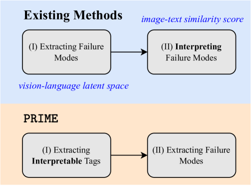
Figure 2: PRIME illustration.

As an example, by running PRIME on a trained model over Living17, we realize that images where a black ape is hanging from a tree branch identify a hard subpopulation such that model’s accuracy drops from 86.23%percent 86.23 86.23%86.23 % to 41.88%percent 41.88 41.88%41.88 %. Crucially, presence of all 3 3 3 3 of these tags is necessary, i.e., when we consider images that have 1 1 1 1 or 2 2 2 2 of these 3 3 3 3 tags, the accuracy of model is higher. Figure3 illustrates these failure modes. We further study the effect of number of tags in Section5.1.

To further validate our method, we examine data unseen during the computation of our failure mode descriptions. We observe that the images that match a failure mode lead the model to similarly struggle. That is, we demonstrate generalizability of our failure modes, crucially, directly from the succinct text descriptions. While reflecting the quality of our descriptions, this allows for bringing in generative models. We validate this claim by generating hard images using some of the failure mode’s descriptions and compare the accuracy of model on them with some other generated images that correspond to easier subpopulations.

Finally, we show that PRIME produces better descriptions for detected failure modes in terms of similarity, coherency, and specificity of descriptions, compared to prior work that does not prioritize interpretability. Evaluating description quality is challenging and typically requires human assessment, which can be impractical for extensive studies. To mitigate that, inspired by CLIPScore (Hessel et al., 2021), we present a suite of three automated metrics that harness vision-language models to evaluate the quality. These metrics quantify both the intra-group image-description similarity and coherency, while also assessing the specificity of descriptions to ensure they are confined to the designated image groups. We mainly observe that due to putting interpretability first and considering different combinations of tags (concepts), we observe improvements in the quality of generated descriptions. We discuss PRIME’s limitations in AppendixA.1.

Summary of Contribution.

1.We propose PRIME to extract and explain failure modes of a model in human-understandable terms by prioritizing interpretability.
2.Using a suite of three automated metrics to evaluate the quality of generated descriptions, we observe improvements in our method compared to strong baselines such as Eyuboglu et al. (2022) and Jain et al. (2022) on various datasets.
3.We advocate for the concept of putting interpretability first by providing empirical evidence derived from latent space analysis, suggesting that distance in latent space may at times be a misleading measure of semantic similarity for explaining model failure modes.

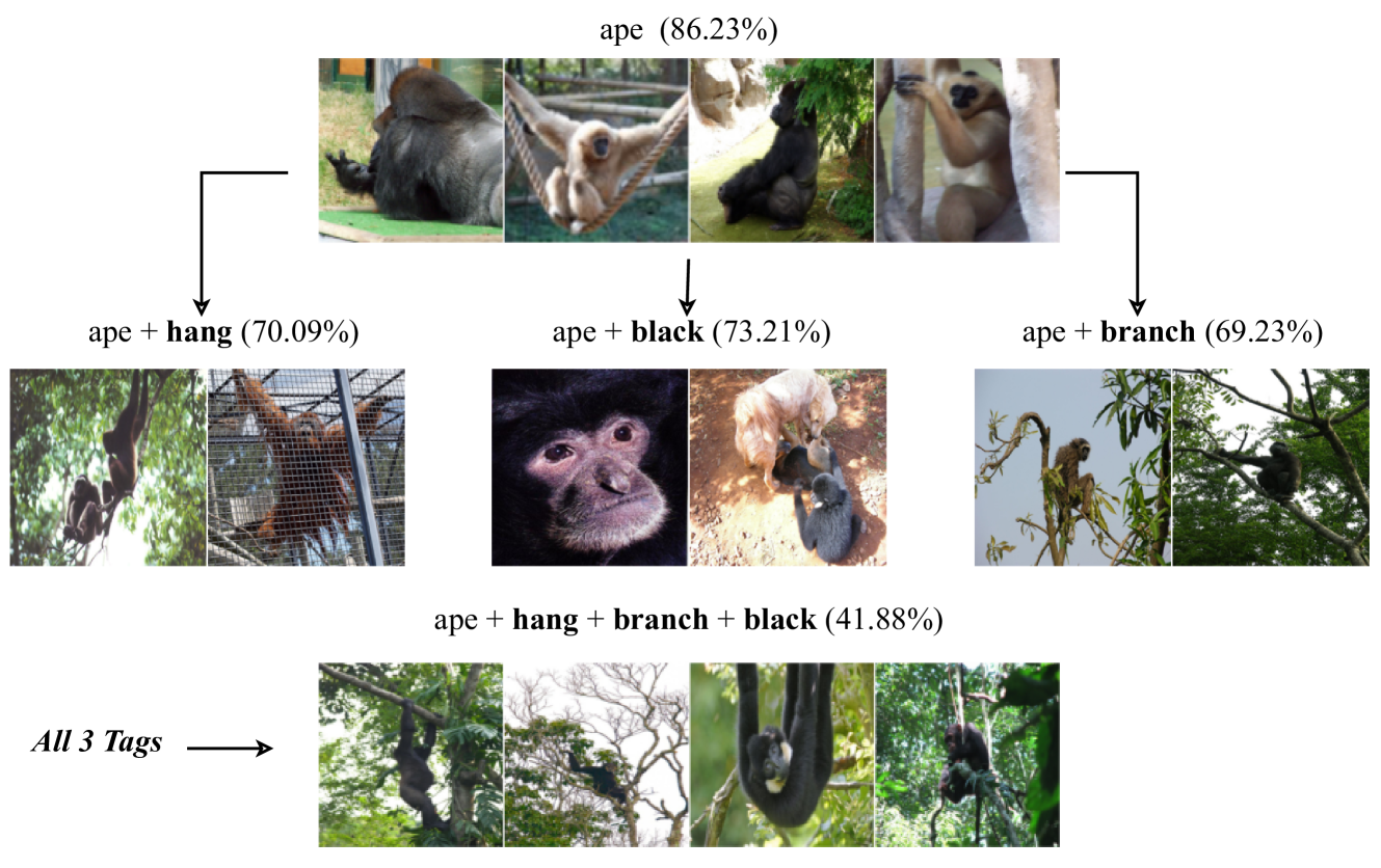
Figure 3: Although appearance of tags “hang”, “black”, and “branch” individually lowers model’s accuracy, when all of them appear in the images, model’s accuracy drops from 86.23%percent 86.23 86.23%86.23 % to 41.88%percent 41.88 41.88%41.88 %.

2 Literature Review

Failure mode discovery. The exploration of biases or challenging subpopulations within datasets, where a model’s performance significantly declines, has been the subject of research in the field. Some recent methods for detecting such biases rely on human intervention, which can be time-consuming and impractical for routine usage. For instance, recent works (Tsipras et al., 2020; Vasudevan et al., 2022) depend on manual data exploration to identify failure modes in widely used datasets like ImageNet. Another line of work uses crowdsourcing (Nushi et al., 2018; Idrissi et al., 2022; Plumb et al., 2021) or simulators (Leclerc et al., 2022) to label visual features, but these methods are expensive and not universally applicable. Some researchers utilize feature visualization (Engstrom et al., 2019; Olah et al., 2017) or saliency maps (Selvaraju et al., 2017; Adebayo et al., 2018) to gain insights into the model’s failure, but these techniques provide information specific to individual samples and lack aggregated knowledge across the entire dataset. Some other approaches (Sohoni et al., 2020a; Nam et al., 2020; Liu et al., 2021; Hashimoto et al., 2018) automatically identify failure modes of a model but do not provide human-understandable descriptions for them.

Recent efforts have been made to identify difficult subpopulations and assign human-understandable descriptions to them (Eyuboglu et al., 2022; Jain et al., 2022; Kim et al., 2023). DOMINO (Eyuboglu et al., 2022) uses the latent representation of images in a vision-language model to cluster difficult images and then assigns human-understandable descriptions to these clusters. Jain et al. (2022) identifies a failure direction in the latent space and assigns description to images aligned with that direction. Hoffmann et al. (2021) shows that there is a semantic gap between similarity in latent space and similarity in input space, which can corrupt the output of methods that rely on assigning descriptions to latent embeddings. In (Kim et al., 2023), concepts are identified whose presence in images leads to a substantial decrease in the model’s accuracy. Recent studies (Johnson et al., 2023; Gao et al., 2023) highlight the challenge of producing high-quality descriptions in the context of failure mode detection.

Vision-Language and Tagging models. Vision-language models have achieved remarkable success through pre-training on large-scale image-text pairs (Radford et al., 2021). These models can be utilized to incorporate vision-language space and evaluate captions generated to describe images. Recently Moayeri et al. (2023); Li et al. (2023) bridge the modality gap and enable off-the-shelf vision encoders to access shared vision-language space. Furthermore, in our method, we utilize models capable of generating tags for input images (Huang et al., 2023; Zhang et al., 2023).

3 Extracting Failure Modes by Conditioning on Human-understandable Tags

Undesirable patterns or spurious correlations within the training dataset can lead to performance discrepancies in the learned models. For instance, in the Waterbirds dataset (Sagawa et al., 2019), images of landbirds are predominantly captured in terrestrial environments such as forests or grasslands. Consequently, a model can heavily rely on the background and make a prediction based on that. Conversely, the model may also rely on cues such as the presence of the ocean, sea, or boats to identify the input as waterbirds. This can result in performance drops for images where a waterbird is photographed on land or a landbird is photographed at sea. Detecting failure modes involves identifying groups of inputs where the model’s performance significantly declines. While locating failure inputs is straightforward, categorizing them into distinct groups characterized by human-understandable concepts is a challenging task. To explain failure modes, we propose PRIME. Our method consists of two steps: (I) obtaining relevant tags for the images, and (II) identifying failure modes based on extracted tags.

3.1 Obtaining Relevant Tags

We start our method by collecting concepts (tags) over the images in the dataset. For example, for a photo of a fox sampled from ImageNet (Deng et al., 2009), we may collect tags “orange”, “grass”, “trees”, “walking”, “zoo”, and others. To generate these tags for each image in our dataset, we employ the state-of-the-art Recognize Anything Model (RAM)(Zhang et al., 2023; Huang et al., 2023), which is a model trained on image-caption pairs to generate tags for the input images. RAM makes a substantial step for large models in computer vision, demonstrating the zero-shot ability to recognize any common category with high accuracy.

Let 𝒟 𝒟\mathcal{D}caligraphic_D be the set of all images. We obtain tags over all images of 𝒟 𝒟\mathcal{D}caligraphic_D. Then, we analyze the effect of tags on prediction in a class-wise manner. In fact, the effect of tags and patterns on the model’s prediction depends on the main object in the images, e.g., presence of water in the background improves performance on images labeled as waterbird while degrading performance on landbird images. For each class c 𝑐 c italic_c in the dataset, we take the union of tags generated by the model over images of class c 𝑐 c italic_c. Subsequently, we eliminate tags that occur less frequently than a predetermined threshold. This threshold varies depending on the dataset size, specifically set at 50 50 50 50, 100 100 100 100, and 200 200 200 200 in our experimental scenarios. In fact, we remove rare (irrelevant) tags and obtain a set of tags T c subscript 𝑇 𝑐 T_{c}italic_T start_POSTSUBSCRIPT italic_c end_POSTSUBSCRIPT for each class c 𝑐 c italic_c in the dataset, e.g., T c={⁢⁢red⁢",⁢⁢orange⁢",⁢⁢snow⁢",⁢⁢grass⁢",…}subscript 𝑇 𝑐red"orange"snow"grass"…T_{c}={\textnormal{red}",\textnormal{orange}",\textnormal{snow}",% \textnormal{grass}",...}italic_T start_POSTSUBSCRIPT italic_c end_POSTSUBSCRIPT = { red " , orange " , snow " , grass " , … }.

3.2 Detecting Failure Modes

After obtaining tags, we mainly focus on tags whose presence in the image leads to a performance drop in the model. Indeed, for each class c 𝑐 c italic_c, we pick a subset S c⊆T c subscript 𝑆 𝑐 subscript 𝑇 𝑐 S_{c}\subseteq T_{c}italic_S start_POSTSUBSCRIPT italic_c end_POSTSUBSCRIPT ⊆ italic_T start_POSTSUBSCRIPT italic_c end_POSTSUBSCRIPT of tags and evaluate the model’s performance on the images of class c 𝑐 c italic_c including all tags in S c subscript 𝑆 𝑐 S_{c}italic_S start_POSTSUBSCRIPT italic_c end_POSTSUBSCRIPT. We denote this set of images by I S c subscript 𝐼 subscript 𝑆 𝑐 I_{S_{c}}italic_I start_POSTSUBSCRIPT italic_S start_POSTSUBSCRIPT italic_c end_POSTSUBSCRIPT end_POSTSUBSCRIPT. I S C subscript 𝐼 subscript 𝑆 𝐶 I_{S_{C}}italic_I start_POSTSUBSCRIPT italic_S start_POSTSUBSCRIPT italic_C end_POSTSUBSCRIPT end_POSTSUBSCRIPT is a coherent image set in the sense that those images share at least the tags in S c subscript 𝑆 𝑐 S_{c}italic_S start_POSTSUBSCRIPT italic_c end_POSTSUBSCRIPT.

For I S c subscript 𝐼 subscript 𝑆 𝑐 I_{S_{c}}italic_I start_POSTSUBSCRIPT italic_S start_POSTSUBSCRIPT italic_c end_POSTSUBSCRIPT end_POSTSUBSCRIPT, to be a failure mode, we require that the model’s accuracy over images of I S c subscript 𝐼 subscript 𝑆 𝑐 I_{S_{c}}italic_I start_POSTSUBSCRIPT italic_S start_POSTSUBSCRIPT italic_c end_POSTSUBSCRIPT end_POSTSUBSCRIPT significantly drops, i.e., denoting the model’s accuracy over images of I S c subscript 𝐼 subscript 𝑆 𝑐 I_{S_{c}}italic_I start_POSTSUBSCRIPT italic_S start_POSTSUBSCRIPT italic_c end_POSTSUBSCRIPT end_POSTSUBSCRIPT by A S c subscript 𝐴 subscript 𝑆 𝑐 A_{S_{c}}italic_A start_POSTSUBSCRIPT italic_S start_POSTSUBSCRIPT italic_c end_POSTSUBSCRIPT end_POSTSUBSCRIPT and the model’s overall accuracy over the images of class c 𝑐 c italic_c by A c subscript 𝐴 𝑐 A_{c}italic_A start_POSTSUBSCRIPT italic_c end_POSTSUBSCRIPT, then A S c≤A c−a subscript 𝐴 subscript 𝑆 𝑐 subscript 𝐴 𝑐 𝑎 A_{S_{c}}\leq A_{c}-a italic_A start_POSTSUBSCRIPT italic_S start_POSTSUBSCRIPT italic_c end_POSTSUBSCRIPT end_POSTSUBSCRIPT ≤ italic_A start_POSTSUBSCRIPT italic_c end_POSTSUBSCRIPT - italic_a. Parameter a 𝑎 a italic_a plays a pivotal role in determining the severity of the failure modes we aim to detect. Importantly, we want the tags in S c subscript 𝑆 𝑐 S_{c}italic_S start_POSTSUBSCRIPT italic_c end_POSTSUBSCRIPT to be minimal, i.e., none of them should be redundant. In order to ensure that, we expect that the removal of any of tags in S c subscript 𝑆 𝑐 S_{c}italic_S start_POSTSUBSCRIPT italic_c end_POSTSUBSCRIPT determines a relatively easier subpopulation. In essence, presence of all tags in S c subscript 𝑆 𝑐 S_{c}italic_S start_POSTSUBSCRIPT italic_c end_POSTSUBSCRIPT is deemed essential to obtain that hard subpopulation.

More precisely, Let n 𝑛 n italic_n to be the cardinality of S c subscript 𝑆 𝑐 S_{c}italic_S start_POSTSUBSCRIPT italic_c end_POSTSUBSCRIPT, i.e., n=|S c|𝑛 subscript 𝑆 𝑐 n=|S_{c}|italic_n = | italic_S start_POSTSUBSCRIPT italic_c end_POSTSUBSCRIPT |. We require all tags t∈S c 𝑡 subscript 𝑆 𝑐 t\in S_{c}italic_t ∈ italic_S start_POSTSUBSCRIPT italic_c end_POSTSUBSCRIPT to be necessary. i.e., if we remove a tag t 𝑡 t italic_t from S c subscript 𝑆 𝑐 S_{c}italic_S start_POSTSUBSCRIPT italic_c end_POSTSUBSCRIPT, then the resulting group of images should become an easier subpopulation. More formally, for all t∈S c 𝑡 subscript 𝑆 𝑐 t\in S_{c}italic_t ∈ italic_S start_POSTSUBSCRIPT italic_c end_POSTSUBSCRIPT, A S c∖t≥A S c+b n subscript 𝐴 subscript 𝑆 𝑐 𝑡 subscript 𝐴 subscript 𝑆 𝑐 subscript 𝑏 𝑛 A_{S_{c}\setminus t}\geq A_{S_{c}}+b_{n}italic_A start_POSTSUBSCRIPT italic_S start_POSTSUBSCRIPT italic_c end_POSTSUBSCRIPT ∖ italic_t end_POSTSUBSCRIPT ≥ italic_A start_POSTSUBSCRIPT italic_S start_POSTSUBSCRIPT italic_c end_POSTSUBSCRIPT end_POSTSUBSCRIPT + italic_b start_POSTSUBSCRIPT italic_n end_POSTSUBSCRIPT where b 2,b 3,b 4,…subscript 𝑏 2 subscript 𝑏 3 subscript 𝑏 4…b_{2},b_{3},b_{4},...italic_b start_POSTSUBSCRIPT 2 end_POSTSUBSCRIPT , italic_b start_POSTSUBSCRIPT 3 end_POSTSUBSCRIPT , italic_b start_POSTSUBSCRIPT 4 end_POSTSUBSCRIPT , … are some hyperparameters that determine the degree of necessity of appearance of all tags in a group. We generally pick b 2=10%subscript 𝑏 2 percent 10 b_{2}=10%italic_b start_POSTSUBSCRIPT 2 end_POSTSUBSCRIPT = 10 %, b 3=5%subscript 𝑏 3 percent 5 b_{3}=5%italic_b start_POSTSUBSCRIPT 3 end_POSTSUBSCRIPT = 5 % and b 4=2.5%subscript 𝑏 4 percent 2.5 b_{4}=2.5%italic_b start_POSTSUBSCRIPT 4 end_POSTSUBSCRIPT = 2.5 % in our experiments. These values help us fine-tune the sensitivity to tag necessity and identify meaningful failure modes. Furthermore, we require a minimum of s 𝑠 s italic_s samples in I S c subscript 𝐼 subscript 𝑆 𝑐 I_{S_{c}}italic_I start_POSTSUBSCRIPT italic_S start_POSTSUBSCRIPT italic_c end_POSTSUBSCRIPT end_POSTSUBSCRIPT for reliability and generalization. This ensures a sufficient number of instances where the model’s performance drops, allowing us to confidently identify failure modes. Figure1 shows some of the obtained failure modes.

How to obtain failure modes. We generally use Exhaustive Search to obtain failure modes. In exhaustive search, we systematically evaluate various combinations of tags to identify failure modes, employing a brute-force approach that covers all possible combinations of tags up to l 𝑙 l italic_l ones. More precisely, we consider all subsets S c⊆T c subscript 𝑆 𝑐 subscript 𝑇 𝑐 S_{c}\subseteq T_{c}italic_S start_POSTSUBSCRIPT italic_c end_POSTSUBSCRIPT ⊆ italic_T start_POSTSUBSCRIPT italic_c end_POSTSUBSCRIPT such that |S c|≤l subscript 𝑆 𝑐 𝑙|S_{c}|\leq l| italic_S start_POSTSUBSCRIPT italic_c end_POSTSUBSCRIPT | ≤ italic_l and evaluate the model’s performance on I S c subscript 𝐼 subscript 𝑆 𝑐 I_{S_{c}}italic_I start_POSTSUBSCRIPT italic_S start_POSTSUBSCRIPT italic_c end_POSTSUBSCRIPT end_POSTSUBSCRIPT. As mentioned above, we detect S c subscript 𝑆 𝑐 S_{c}italic_S start_POSTSUBSCRIPT italic_c end_POSTSUBSCRIPT as a failure mode if (1) |I S c|≥s subscript 𝐼 subscript 𝑆 𝑐 𝑠|I_{S_{c}}|\geq s| italic_I start_POSTSUBSCRIPT italic_S start_POSTSUBSCRIPT italic_c end_POSTSUBSCRIPT end_POSTSUBSCRIPT | ≥ italic_s, (2) model’s accuracy over I S c subscript 𝐼 subscript 𝑆 𝑐 I_{S_{c}}italic_I start_POSTSUBSCRIPT italic_S start_POSTSUBSCRIPT italic_c end_POSTSUBSCRIPT end_POSTSUBSCRIPT is at most A c−a subscript 𝐴 𝑐 𝑎 A_{c}-a italic_A start_POSTSUBSCRIPT italic_c end_POSTSUBSCRIPT - italic_a, and (3) S c subscript 𝑆 𝑐 S_{c}italic_S start_POSTSUBSCRIPT italic_c end_POSTSUBSCRIPT is minimal, i.e., for all t∈S c 𝑡 subscript 𝑆 𝑐 t\in S_{c}italic_t ∈ italic_S start_POSTSUBSCRIPT italic_c end_POSTSUBSCRIPT, A S c∖t≥A S c+b|S c|subscript 𝐴 subscript 𝑆 𝑐 𝑡 subscript 𝐴 subscript 𝑆 𝑐 subscript 𝑏 subscript 𝑆 𝑐 A_{S_{c}\setminus t}\geq A_{S_{c}}+b_{|S_{c}|}italic_A start_POSTSUBSCRIPT italic_S start_POSTSUBSCRIPT italic_c end_POSTSUBSCRIPT ∖ italic_t end_POSTSUBSCRIPT ≥ italic_A start_POSTSUBSCRIPT italic_S start_POSTSUBSCRIPT italic_c end_POSTSUBSCRIPT end_POSTSUBSCRIPT + italic_b start_POSTSUBSCRIPT | italic_S start_POSTSUBSCRIPT italic_c end_POSTSUBSCRIPT | end_POSTSUBSCRIPT. It is worth noting that the final output of the method is all sets I S c subscript 𝐼 subscript 𝑆 𝑐 I_{S_{c}}italic_I start_POSTSUBSCRIPT italic_S start_POSTSUBSCRIPT italic_c end_POSTSUBSCRIPT end_POSTSUBSCRIPT that satisfy those conditions and description for this group consist of class name (c 𝑐 c italic_c) and all tags in S c subscript 𝑆 𝑐 S_{c}italic_S start_POSTSUBSCRIPT italic_c end_POSTSUBSCRIPT.

We note that the aforementioned method runs with a complexity of O⁢(|T c|l⁢|𝒟|)𝑂 superscript subscript 𝑇 𝑐 𝑙 𝒟 O\left(|T_{c}|^{l}|\mathcal{D}|\right)italic_O ( | italic_T start_POSTSUBSCRIPT italic_c end_POSTSUBSCRIPT | start_POSTSUPERSCRIPT italic_l end_POSTSUPERSCRIPT | caligraphic_D | ). However, l 𝑙 l italic_l is generally small, i.e., for a failure mode to be generalizable, we mainly consider cases where l≤4 𝑙 4 l\leq 4 italic_l ≤ 4. Furthermore, in our experiments over different datasets |T c|≈100 subscript 𝑇 𝑐 100|T_{c}|\approx 100| italic_T start_POSTSUBSCRIPT italic_c end_POSTSUBSCRIPT | ≈ 100, thus, the exhaustive search is relatively efficient. For instance, running exhaustive search (l=4,s=30,a=30%formulae-sequence 𝑙 4 formulae-sequence 𝑠 30 𝑎 percent 30 l=4,s=30,a=30%italic_l = 4 , italic_s = 30 , italic_a = 30 %) on Living17 dataset having 17 17 17 17 classes with 88400 88400 88400 88400 images results in obtaining 132 132 132 132 failure modes within a time frame of under 5 5 5 5 minutes. We refer to AppendixA.6 for more efficient algorithms and AppendixA.15 for more detailed explanation of PRIME’s hyperparameters.

Experiments and Comparison to Existing Work. We run experiments on models trained on Living17, NonLiving26, Entity13 (Santurkar et al., 2020), Waterbirds (Sagawa et al., 2019), and CelebA (Liu et al., 2015) (for age classification). We refer to AppendixA.2 for model training details and the different hyperparameters we used for failure mode detection. We refer to AppendixA.3 for the full results of our method on different datasets. We engage two of the most recent failure mode detection approaches DOMINO(Eyuboglu et al., 2022) and Distilling Failure Directions(Jain et al., 2022) as strong baselines and compare our approach with them.

4 Evaluation

Let 𝒟 𝒟\mathcal{D}caligraphic_D be the dataset on which we detect failure modes of a trained model. The result of a human-understandable failure mode extractor on this dataset consists of sets of images, denoted as I 1,I 2,…,I m subscript 𝐼 1 subscript 𝐼 2…subscript 𝐼 𝑚 I_{1},I_{2},...,I_{m}italic_I start_POSTSUBSCRIPT 1 end_POSTSUBSCRIPT , italic_I start_POSTSUBSCRIPT 2 end_POSTSUBSCRIPT , … , italic_I start_POSTSUBSCRIPT italic_m end_POSTSUBSCRIPT, along with corresponding descriptions, labeled as T 1,T 2,…,T m subscript 𝑇 1 subscript 𝑇 2…subscript 𝑇 𝑚 T_{1},T_{2},...,T_{m}italic_T start_POSTSUBSCRIPT 1 end_POSTSUBSCRIPT , italic_T start_POSTSUBSCRIPT 2 end_POSTSUBSCRIPT , … , italic_T start_POSTSUBSCRIPT italic_m end_POSTSUBSCRIPT. Each set I j subscript 𝐼 𝑗 I_{j}italic_I start_POSTSUBSCRIPT italic_j end_POSTSUBSCRIPT comprises images that share similar attributes, leading to a noticeable drop in model accuracy. Number of detected failure modes, m 𝑚 m italic_m, is influenced by various hyperparameters, e.g., in our method, minimum accuracy drop (a 𝑎 a italic_a), values for b 2,b 3,…subscript 𝑏 2 subscript 𝑏 3…b_{2},b_{3},...italic_b start_POSTSUBSCRIPT 2 end_POSTSUBSCRIPT , italic_b start_POSTSUBSCRIPT 3 end_POSTSUBSCRIPT , …, and the minimum group size (s 𝑠 s italic_s) are these parameters.

One of the main goals of detecting failure modes in human-understandable terms is to generate high-quality captions for hard subpopulations. We note that these methods should also be evaluated in terms of coverage, i.e., what portion of failure inputs are covered along with the performance gap in detected failure modes. All these methods extract hard subpopulations on which the model’s accuracy significantly drops, and coverage depends on the dataset and the hyperparameters of the method, thus, we mainly focus on generalizability of our approach and quality of descriptions.

4.1 Generalization on Unseen Data

In order to evaluate generalizability of the resulted descriptions, we take dataset 𝒟′superscript 𝒟′\mathcal{D^{\prime}}caligraphic_D start_POSTSUPERSCRIPT ′ end_POSTSUPERSCRIPT including unseen images and recover relevant images in that to each of captions T 1,T 2,…,T m subscript 𝑇 1 subscript 𝑇 2…subscript 𝑇 𝑚 T_{1},T_{2},...,T_{m}italic_T start_POSTSUBSCRIPT 1 end_POSTSUBSCRIPT , italic_T start_POSTSUBSCRIPT 2 end_POSTSUBSCRIPT , … , italic_T start_POSTSUBSCRIPT italic_m end_POSTSUBSCRIPT, thus, obtaining I 1′,I 2′,…,I m′subscript superscript 𝐼′1 subscript superscript 𝐼′2…subscript superscript 𝐼′𝑚 I^{\prime}{1},I^{\prime}{2},...,I^{\prime}{m}italic_I start_POSTSUPERSCRIPT ′ end_POSTSUPERSCRIPT start_POSTSUBSCRIPT 1 end_POSTSUBSCRIPT , italic_I start_POSTSUPERSCRIPT ′ end_POSTSUPERSCRIPT start_POSTSUBSCRIPT 2 end_POSTSUBSCRIPT , … , italic_I start_POSTSUPERSCRIPT ′ end_POSTSUPERSCRIPT start_POSTSUBSCRIPT italic_m end_POSTSUBSCRIPT. Indeed, I j′subscript superscript 𝐼′𝑗 I^{\prime}{j}italic_I start_POSTSUPERSCRIPT ′ end_POSTSUPERSCRIPT start_POSTSUBSCRIPT italic_j end_POSTSUBSCRIPT includes images in 𝒟′superscript 𝒟′\mathcal{D^{\prime}}caligraphic_D start_POSTSUPERSCRIPT ′ end_POSTSUPERSCRIPT that are relevant to T j subscript 𝑇 𝑗 T_{j}italic_T start_POSTSUBSCRIPT italic_j end_POSTSUBSCRIPT. If captions can describe hard subpopulations, then we expect hard subpopulations in I 1′,I 2′,…,I m′subscript superscript 𝐼′1 subscript superscript 𝐼′2…subscript superscript 𝐼′𝑚 I^{\prime}{1},I^{\prime}{2},...,I^{\prime}{m}italic_I start_POSTSUPERSCRIPT ′ end_POSTSUPERSCRIPT start_POSTSUBSCRIPT 1 end_POSTSUBSCRIPT , italic_I start_POSTSUPERSCRIPT ′ end_POSTSUPERSCRIPT start_POSTSUBSCRIPT 2 end_POSTSUBSCRIPT , … , italic_I start_POSTSUPERSCRIPT ′ end_POSTSUPERSCRIPT start_POSTSUBSCRIPT italic_m end_POSTSUBSCRIPT. Additionally, since 𝒟 𝒟\mathcal{D}caligraphic_D and 𝒟′superscript 𝒟′\mathcal{D^{\prime}}caligraphic_D start_POSTSUPERSCRIPT ′ end_POSTSUPERSCRIPT share the same distribution, we anticipate the accuracy drop in I j subscript 𝐼 𝑗 I{j}italic_I start_POSTSUBSCRIPT italic_j end_POSTSUBSCRIPT to closely resemble that in I j′subscript superscript 𝐼′𝑗 I^{\prime}_{j}italic_I start_POSTSUPERSCRIPT ′ end_POSTSUPERSCRIPT start_POSTSUBSCRIPT italic_j end_POSTSUBSCRIPT.

In our method, for a detected failure mode I S c subscript 𝐼 subscript 𝑆 𝑐 I_{S_{c}}italic_I start_POSTSUBSCRIPT italic_S start_POSTSUBSCRIPT italic_c end_POSTSUBSCRIPT end_POSTSUBSCRIPT, we obtain I S c′subscript superscript 𝐼′subscript 𝑆 𝑐 I^{\prime}{S{c}}italic_I start_POSTSUPERSCRIPT ′ end_POSTSUPERSCRIPT start_POSTSUBSCRIPT italic_S start_POSTSUBSCRIPT italic_c end_POSTSUBSCRIPT end_POSTSUBSCRIPT by collecting images of 𝒟′superscript 𝒟′\mathcal{D^{\prime}}caligraphic_D start_POSTSUPERSCRIPT ′ end_POSTSUPERSCRIPT that have all tags in S c subscript 𝑆 𝑐 S_{c}italic_S start_POSTSUBSCRIPT italic_c end_POSTSUBSCRIPT. For example, if appearance of tags “black”, “snowing”, and “forest” is detected as a failure mode for class “bear”, we evaluate model’s performance on images of “bear” in 𝒟′superscript 𝒟′\mathcal{D^{\prime}}caligraphic_D start_POSTSUPERSCRIPT ′ end_POSTSUPERSCRIPT that include those three tags, expecting a significant accuracy drop for model on those images. As seen in Figure9, PRIME shows a good level of generalizability. We refer to AppendixA.5 for generalization on other datasets with respect to different hyperparameters (s 𝑠 s italic_s and a 𝑎 a italic_a). While all our detected failure modes generalize well, we observe stronger generalization when using more stringent hyperparameter values (high s 𝑠 s italic_s and a 𝑎 a italic_a), though it comes at the cost of detecting fewer modes.

Figure 4: Accuracy of model over 50 50 50 50 generated images corresponding to one of the success modes and failure modes for classes “bear”, “ parrot”, and “fox” from Living17. Accuracy gap shows that our method can identify hard and easy subpopulations. Images show that extracted tags are capable of describing detailed images.

In contrast, existing methods (Eyuboglu et al., 2022; Jain et al., 2022) do not provide a direct way to assess generalization from text descriptions alone. See AppendixA.9 for more details.

4.2 Generalization on Generated Data

In this section we validate PRIME on synthetic images. To utilize image generation models, we employ language models to create descriptive captions for objects and tags associated with failure modes in images. We note that use of language models is just for validation on synthetic images, it is not a part of PRIME framework. We discuss about limitations of using language models in AppendixA.1. These captions serve as prompts for text-to-image generative models, enabling the creation of artificial images that correspond to the identified failure modes. To achieve this, we adopt the methodology outlined in Vendrow et al. (2023), which leverages a denoising diffusion model (Ho et al., 2020; Rombach et al., 2022). We fine-tune the generative model on the Living17 dataset to generate images that match the distribution of the data that the classifiers is trained on.

For each class in Living17 dataset, we apply our approach to identify two failure modes (hard subpopulations) and two success modes (easy subpopulations). We then employ ChatGPT 1 1 1 ChatGPT 3.5, August 3 version to generate descriptive captions for these groups. Subsequently, we generate 50 50 50 50 images for each caption and assess the model’s accuracy on these newly generated images. We refer to AppendixA.10 for more details on this experiment and average discrepancy in accuracy between the success modes and failure modes which further validates PRIME. Figure4 provides both accuracy metrics and sample images for three hard and three easy subpopulations.

4.3 Quality of Descriptions

Within this section, our aim is to evaluate the quality of the descriptions for the identified failure modes. In contrast to Section4.2, where language models were employed to create sentence descriptions using the tags associated with each failure mode, here we combine tags and class labels in a bag-of-words manner. For instance, when constructing the description for a failure mode in the “ape” class with the tags “black” + “branch,” we formulate it as ”a photo of ape black branch”. We discuss more about it in AppendixA.1.

In order to evaluate the quality of descriptions, we propose a suite of three complementary automated metrics that utilize vision-language models (such as CLIP) as a proxy to obtain image-text similarity (Hessel et al., 2021). Let t 𝑡 t italic_t be the failure mode’s description, f text⁢(t)subscript 𝑓 text 𝑡 f_{\text{text}}(t)italic_f start_POSTSUBSCRIPT text end_POSTSUBSCRIPT ( italic_t ) denote the normalized embedding of text prompt t 𝑡 t italic_t and f vision⁢(x)subscript 𝑓 vision 𝑥 f_{\text{vision}}(x)italic_f start_POSTSUBSCRIPT vision end_POSTSUBSCRIPT ( italic_x ) denote the normalized embedding of an image x 𝑥 x italic_x. The similarity of image x 𝑥 x italic_x to this failure mode’s description t 𝑡 t italic_t is the dot product of image and text representation in shared vision-language space. More precisely, sim⁢(x,t):=⟨f vision⁢(x),f text⁢(t)⟩assign sim 𝑥 𝑡 subscript 𝑓 vision 𝑥 subscript 𝑓 text 𝑡\text{sim}(x,t):=\langle f_{\text{vision}}(x),f_{\text{text}}(t)\rangle sim ( italic_x , italic_t ) := ⟨ italic_f start_POSTSUBSCRIPT vision end_POSTSUBSCRIPT ( italic_x ) , italic_f start_POSTSUBSCRIPT text end_POSTSUBSCRIPT ( italic_t ) ⟩.

For a high-quality failure mode I j subscript 𝐼 𝑗 I_{j}italic_I start_POSTSUBSCRIPT italic_j end_POSTSUBSCRIPT and its description T j subscript 𝑇 𝑗 T_{j}italic_T start_POSTSUBSCRIPT italic_j end_POSTSUBSCRIPT, we wish T j subscript 𝑇 𝑗 T_{j}italic_T start_POSTSUBSCRIPT italic_j end_POSTSUBSCRIPT to be similar to images in I j subscript 𝐼 𝑗 I_{j}italic_I start_POSTSUBSCRIPT italic_j end_POSTSUBSCRIPT, thus, we consider the average similarity of images in I j subscript 𝐼 𝑗 I_{j}italic_I start_POSTSUBSCRIPT italic_j end_POSTSUBSCRIPT and T j subscript 𝑇 𝑗 T_{j}italic_T start_POSTSUBSCRIPT italic_j end_POSTSUBSCRIPT. we further expect a high level of coherency among all images in I j subscript 𝐼 𝑗 I_{j}italic_I start_POSTSUBSCRIPT italic_j end_POSTSUBSCRIPT, i.e., these images should all share multiple semantic attributes described by text, thus, we wish the standard deviation of similarity scores between images in I j subscript 𝐼 𝑗 I_{j}italic_I start_POSTSUBSCRIPT italic_j end_POSTSUBSCRIPT and T j subscript 𝑇 𝑗 T_{j}italic_T start_POSTSUBSCRIPT italic_j end_POSTSUBSCRIPT to be low. Lastly, we expect generated captions to be specific, capturing the essence of the failure mode, without including distracting irrelevant information. That is, caption T j subscript 𝑇 𝑗 T_{j}italic_T start_POSTSUBSCRIPT italic_j end_POSTSUBSCRIPT should only describe images in I j subscript 𝐼 𝑗 I_{j}italic_I start_POSTSUBSCRIPT italic_j end_POSTSUBSCRIPT and not images outside of that. As a result, we consider the AUROC between the similarity score of images inside the failure mode (I j)subscript 𝐼 𝑗(I_{j})( italic_I start_POSTSUBSCRIPT italic_j end_POSTSUBSCRIPT ) and some randomly sampled images outside of that. We note that in existing methods as well as our method, all images in a failure mode have the same label, so we sample from images outside of the group but with the same label.

In Figure5, we show (1) the average similarity score, i.e., for all I j subscript 𝐼 𝑗 I_{j}italic_I start_POSTSUBSCRIPT italic_j end_POSTSUBSCRIPT and x∈I j 𝑥 subscript 𝐼 𝑗 x\in I_{j}italic_x ∈ italic_I start_POSTSUBSCRIPT italic_j end_POSTSUBSCRIPT, we take the mean of sim⁢(x,T j)sim 𝑥 subscript 𝑇 𝑗\text{sim}(x,T_{j})sim ( italic_x , italic_T start_POSTSUBSCRIPT italic_j end_POSTSUBSCRIPT ), (2) the standard deviation of similarity score, i.e., the standard deviation of sim⁢(x,T j)sim 𝑥 subscript 𝑇 𝑗\text{sim}(x,T_{j})sim ( italic_x , italic_T start_POSTSUBSCRIPT italic_j end_POSTSUBSCRIPT ) for all I j subscript 𝐼 𝑗 I_{j}italic_I start_POSTSUBSCRIPT italic_j end_POSTSUBSCRIPT and x∈I j 𝑥 subscript 𝐼 𝑗 x\in I_{j}italic_x ∈ italic_I start_POSTSUBSCRIPT italic_j end_POSTSUBSCRIPT, and (3) the AUROC between the similarity scores of images inside failure modes to their corresponding description and some randomly sampled images outside of the failure mode to that. As shown in Figure5, PRIME improves over DOMINO (Eyuboglu et al., 2022) in terms of all AUROC, average similarity, and standard deviation on different datasets. It is worth noting that this improvement comes even though DOMINO chooses a text caption for the failure mode to maximize the similarity score in latent space. We use hyperparameters for DOMINO to obtain fairly the same number of failure modes detected by PRIME. Results in Figure5 show that PRIME is better than DOMINO in the descriptions it provides for detected failure modes. In AppendixA.8 we provide more details on these experiments. Due to the limitations of Jain et al. (2022) for automatically generating captions, we cannot conduct extensive experiments on various datasets. More details and results on that can be found in AppendixA.11.

5 On Complexity of Failure Mode Explanations

Figure 5: The mean and standard deviation of similarity scores between images in failure modes and their respective descriptions, along with the AUROC measuring the similarity score between descriptions and images inside and outside of failure modes, demonstrate that our method outperforms DOMINO in descriptions it generates for detected failure modes across various datasets.

We note that the main advantage of our method is its more faithful interpretation of failure modes. This comes due to (1) putting interpretability first, i.e., we start by assigning interpretable tags to images and then recognize hard subpopulations and (2) considering combination of several tags which leads to a higher number of attributes (tags) in the description of the group.

5.1 Do We Need to Consider Combination of Tags?

We shed light on the number of tags in the failure modes detected by our approach. We note that unlike Bias2Text (Kim et al., 2023) that finds biased concepts on which model’s behavior changes, we observe that sometimes appearance of several tags (concepts) all together leads to a severe failure mode. As an example, we refer to Table2 where we observe that appearance of all 3 3 3 3 tags together leads to a significant drop while single tags and pairs of them show relatively better performance.

Table 1: Accuracy on unseen images (𝒟′superscript 𝒟′\mathcal{D^{\prime}}caligraphic_D start_POSTSUPERSCRIPT ′ end_POSTSUPERSCRIPT) for class “ape” when given tags appear in the inputs (see Table5 for visualization).

Table 2: Average accuracy drop over unseen images (𝒟′superscript 𝒟′\mathcal{D^{\prime}}caligraphic_D start_POSTSUPERSCRIPT ′ end_POSTSUPERSCRIPT) on failure modes with 3 3 3 3 tags and images have at least 2 2 2 2 of those tags or at least one of them.

In PRIME, we emphasize the necessity of tags. Specifically, for any detected failure mode, the removal of any tag would result in an easier subpopulation. Consequently, failure modes with more tags not only provide more detailed description of their images but also characterize more challenging subpopulations. Table2 presents the average accuracy drop on unseen images for groups identified by three tags, compared to the average accuracy drop on groups identified by subsets of two tags or even a single tag from those failure modes. These results clearly demonstrate that involving more tags leads to the detection of more challenging subpopulations.

5.2 Clustering-Based Methods may Struggle in Generating Coherent Output

Table 3: Statistics of the distance between two points in CelebA conditioned on number of shared tags. Distances are reported using CLIP ViT-B/16 representation space. The last column shows the probability that the distance between two sampled images with at least d 𝑑 d italic_d common tags be more than that of two randomly sampled images.

We empirically analyze the reverse direction of detecting human-understandable failure modes. We note that in recent work where the goal is to obtain interpretable failure modes, those groups are found by clustering images in the latent space. Then, when a group of images or a direction in the latent space is found, these methods leverage the shared space of vision-language to find the text that best describes the images inside the group.

We argue that these approaches, based on distance-based clusters in the representation space, may produce less detailed descriptions. This is because the representation space doesn’t always align perfectly with the semantic space. Even points close to each other in the feature space may differ in certain attributes, and conversely, points sharing human-understandable attributes may not be proximate in the feature space. Hence, these approaches cannot generate high-quality descriptions as their detected clusters in the representation space may contain images with other semantic attributes.

To empirically test this idea, we use two attribute-rich datasets: CelebA (Liu et al., 2015) and CUB-200 (Wah et al., 2011). CelebA features 40 40 40 40 human-understandable tags per image, while CUB-200, a dataset of birds, includes 312 312 312 312 tags per image, all referring to semantic attributes. We use CLIP ViT-B/16 (Radford et al., 2021) and examine its representation space in terms of datasets’ tags. Table3 shows the statistics of the distance between the points conditioned on the number of shared tags. As seen in the Table3, although the average of distance between points with more common tags slightly decreases, the standard deviation of distance between points is high. In fact, points with many common tags can still be far away from each other. Last column in Table3 shows the probability that the distance between two points with at least d 𝑑 d italic_d shared tags be larger than the distance of two randomly sampled points. Even when at least 5 5 5 5 tags are shared between two points, with the probability of 0.34 0.34 0.34 0.34, the distance can be larger than two random points. Thus, if we plant a failure mode on a group of images sharing a subset of tags, these clustering-based methods cannot find a group consisting of only those images; they will inevitably include other irrelevant images, leading to an incoherent failure mode set and, consequently, a low-quality description. This can be observed in AppendixA.7 where we include DOMINO’s output.

We also run another experiment to foster our hypothesis that distance-based clustering methods cannot fully capture semantic similarities. We randomly pick an image x 𝑥 x italic_x and find N 𝑁 N italic_N closest images to x 𝑥 x italic_x in the feature space. Let C 𝐶 C italic_C be the set of these images. We inspect this set in terms of the number of tags that commonly appear in its images as recent methods (Eyuboglu et al., 2022; d’Eon et al., 2021; Jain et al., 2022), take the average embedding of images in C 𝐶 C italic_C and then assign a text to describe images of C 𝐶 C italic_C. Table6 shows the average number of tags that appear in at least α⁢N 𝛼 𝑁\alpha N italic_α italic_N images of set C 𝐶 C italic_C (we sample many different points x 𝑥 x italic_x). If representation space is a good proxy for semantic space, then we expect a large number of shared tags in close proximity to point x 𝑥 x italic_x. At the same time, for the point x 𝑥 x italic_x, we find the maximum number of tags that appear in x 𝑥 x italic_x and at least N 𝑁 N italic_N other images. This is the number of shared tags in close proximity of point x 𝑥 x italic_x but in semantic space. As shown in Table6, average number of shared tags in semantic space is significantly larger than the average number of shared tags in representation space.

6 Conclusions

In this study, drawing from the observation that current techniques in human-comprehensible failure mode detection sometimes produce incoherent descriptions, along with empirical findings related to the latent space of vision-language models, we introduced PRIME, a novel approach that prioritizes interpretability in failure mode detection. Our results demonstrate that it generates descriptions that are more similar, coherent, and specific compared to existing methods for the detected failure modes.

Acknowledgments

This project was supported in part by a grant from an NSF CAREER AWARD 1942230, ONR YIP award N00014-22-1-2271, ARO’s Early Career Program Award 310902-00001, Meta grant 23010098, HR00112090132 (DARPA/RED), HR001119S0026 (DARPA/GARD), Army Grant No. W911NF2120076, NIST 60NANB20D134, the NSF award CCF2212458, an Amazon Research Award and an award from Capital One.

References

Adebayo et al. (2018) Julius Adebayo, Justin Gilmer, Michael Muelly, Ian Goodfellow, Moritz Hardt, and Been Kim. Sanity checks for saliency maps. Advances in neural information processing systems, 31, 2018.
Buolamwini & Gebru (2018) Joy Buolamwini and Timnit Gebru. Gender shades: Intersectional accuracy disparities in commercial gender classification. In Conference on fairness, accountability and transparency, pp. 77–91. PMLR, 2018.
Caron et al. (2021) Mathilde Caron, Hugo Touvron, Ishan Misra, Hervé Jégou, Julien Mairal, Piotr Bojanowski, and Armand Joulin. Emerging properties in self-supervised vision transformers. In Proceedings of the International Conference on Computer Vision (ICCV), 2021.
Deng et al. (2009) Jia Deng, Wei Dong, Richard Socher, Li-Jia Li, Kai Li, and Li Fei-Fei. Imagenet: A large-scale hierarchical image database. In 2009 IEEE conference on computer vision and pattern recognition, pp. 248–255. Ieee, 2009.
d’Eon et al. (2021) Greg d’Eon, Jason d’Eon, James R. Wright, and Kevin Leyton-Brown. The spotlight: A general method for discovering systematic errors in deep learning models, 2021.
Engstrom et al. (2019) Logan Engstrom, Andrew Ilyas, Shibani Santurkar, Dimitris Tsipras, Brandon Tran, and Aleksander Madry. Adversarial robustness as a prior for learned representations. arXiv preprint arXiv:1906.00945, 2019.
Eyuboglu et al. (2022) Sabri Eyuboglu, Maya Varma, Khaled Saab, Jean-Benoit Delbrouck, Christopher Lee-Messer, Jared Dunnmon, James Zou, and Christopher Ré. Domino: Discovering systematic errors with cross-modal embeddings, 2022.
Gao et al. (2023) Irena Gao, Gabriel Ilharco, Scott Lundberg, and Marco Tulio Ribeiro. Adaptive testing of computer vision models, 2023.
Hashimoto et al. (2018) Tatsunori Hashimoto, Megha Srivastava, Hongseok Namkoong, and Percy Liang. Fairness without demographics in repeated loss minimization. In International Conference on Machine Learning, pp.1929–1938. PMLR, 2018.
He et al. (2015) Kaiming He, Xiangyu Zhang, Shaoqing Ren, and Jian Sun. Deep residual learning for image recognition, 2015.
Hessel et al. (2021) Jack Hessel, Ari Holtzman, Maxwell Forbes, Ronan Le Bras, and Yejin Choi. Clipscore: A reference-free evaluation metric for image captioning. ArXiv, abs/2104.08718, 2021. URL https://api.semanticscholar.org/CorpusID:233296711.
Ho et al. (2020) Jonathan Ho, Ajay Jain, and Pieter Abbeel. Denoising diffusion probabilistic models. Advances in neural information processing systems, 33:6840–6851, 2020.
Hoffmann et al. (2021) Adrian Hoffmann, Claudio Fanconi, Rahul Rade, and Jonas Moritz Kohler. This looks like that… does it? shortcomings of latent space prototype interpretability in deep networks. ArXiv, abs/2105.02968, 2021. URL https://api.semanticscholar.org/CorpusID:234094683.
Huang et al. (2023) Xinyu Huang, Youcai Zhang, Jinyu Ma, Weiwei Tian, Rui Feng, Yuejie Zhang, Yaqian Li, Yandong Guo, and Lei Zhang. Tag2text: Guiding vision-language model via image tagging. arXiv preprint arXiv:2303.05657, 2023.
Idrissi et al. (2022) Badr Youbi Idrissi, Diane Bouchacourt, Randall Balestriero, Ivan Evtimov, Caner Hazirbas, Nicolas Ballas, Pascal Vincent, Michal Drozdzal, David Lopez-Paz, and Mark Ibrahim. Imagenet-x: Understanding model mistakes with factor of variation annotations. arXiv preprint arXiv:2211.01866, 2022.
Jain et al. (2022) Saachi Jain, Hannah Lawrence, Ankur Moitra, and Aleksander Madry. Distilling model failures as directions in latent space, 2022.
Johnson et al. (2023) Nari Johnson, Ángel Alexander Cabrera, Gregory Plumb, and Ameet Talwalkar. Where does my model underperform? a human evaluation of slice discovery algorithms, 2023.
Kattakinda et al. (2022) Priyatham Kattakinda, Alexander Levine, and Soheil Feizi. Invariant learning via diffusion dreamed distribution shifts. arXiv preprint arXiv:2211.10370, 2022.
Kim et al. (2019) Michael P Kim, Amirata Ghorbani, and James Zou. Multiaccuracy: Black-box post-processing for fairness in classification. In Proceedings of the 2019 AAAI/ACM Conference on AI, Ethics, and Society, pp. 247–254, 2019.
Kim et al. (2023) Younghyun Kim, Sangwoo Mo, Minkyu Kim, Kyungmin Lee, Jaeho Lee, and Jinwoo Shin. Bias-to-text: Debiasing unknown visual biases through language interpretation, 2023.
Leclerc et al. (2022) Guillaume Leclerc, Hadi Salman, Andrew Ilyas, Sai Vemprala, Logan Engstrom, Vibhav Vineet, Kai Xiao, Pengchuan Zhang, Shibani Santurkar, Greg Yang, et al. 3db: A framework for debugging computer vision models. Advances in Neural Information Processing Systems, 35:8498–8511, 2022.
Li et al. (2023) Junnan Li, Dongxu Li, Silvio Savarese, and Steven Hoi. Blip-2: Bootstrapping language-image pre-training with frozen image encoders and large language models. arXiv preprint arXiv:2301.12597, 2023.
Liu et al. (2021) Evan Z Liu, Behzad Haghgoo, Annie S Chen, Aditi Raghunathan, Pang Wei Koh, Shiori Sagawa, Percy Liang, and Chelsea Finn. Just train twice: Improving group robustness without training group information. In International Conference on Machine Learning, pp.6781–6792. PMLR, 2021.
Liu et al. (2015) Ziwei Liu, Ping Luo, Xiaogang Wang, and Xiaoou Tang. Deep learning face attributes in the wild. In Proceedings of International Conference on Computer Vision (ICCV), December 2015.
Moayeri et al. (2023) Mazda Moayeri, Keivan Rezaei, Maziar Sanjabi, and Soheil Feizi. Text-to-concept (and back) via cross-model alignment. arXiv preprint arXiv:2305.06386, 2023.
Nam et al. (2020) Junhyun Nam, Hyuntak Cha, Sungsoo Ahn, Jaeho Lee, and Jinwoo Shin. Learning from failure: De-biasing classifier from biased classifier. Advances in Neural Information Processing Systems, 33:20673–20684, 2020.
Nushi et al. (2018) Besmira Nushi, Ece Kamar, and Eric Horvitz. Towards accountable ai: Hybrid human-machine analyses for characterizing system failure. In Proceedings of the AAAI Conference on Human Computation and Crowdsourcing, volume 6, pp. 126–135, 2018.
Olah et al. (2017) Chris Olah, Alexander Mordvintsev, and Ludwig Schubert. Feature visualization. Distill, 2(11):e7, 2017.
Plumb et al. (2021) Gregory Plumb, Marco Tulio Ribeiro, and Ameet Talwalkar. Finding and fixing spurious patterns with explanations. arXiv preprint arXiv:2106.02112, 2021.
Radford et al. (2021) Alec Radford, Jong Wook Kim, Chris Hallacy, Aditya Ramesh, Gabriel Goh, Sandhini Agarwal, Girish Sastry, Amanda Askell, Pamela Mishkin, Jack Clark, et al. Learning transferable visual models from natural language supervision. In International conference on machine learning, pp.8748–8763. PMLR, 2021.
Ramesh et al. (2022) Aditya Ramesh, Prafulla Dhariwal, Alex Nichol, Casey Chu, and Mark Chen. Hierarchical text-conditional image generation with clip latents. arXiv preprint arXiv:2204.06125, 1(2):3, 2022.
Rombach et al. (2022) Robin Rombach, Andreas Blattmann, Dominik Lorenz, Patrick Esser, and Björn Ommer. High-resolution image synthesis with latent diffusion models. In Proceedings of the IEEE/CVF conference on computer vision and pattern recognition, pp. 10684–10695, 2022.
Sagawa et al. (2019) Shiori Sagawa, Pang Wei Koh, Tatsunori B. Hashimoto, and Percy Liang. Distributionally robust neural networks for group shifts: On the importance of regularization for worst-case generalization. CoRR, abs/1911.08731, 2019. URL http://arxiv.org/abs/1911.08731.
Saharia et al. (2022) Chitwan Saharia, William Chan, Saurabh Saxena, Lala Li, Jay Whang, Emily L Denton, Kamyar Ghasemipour, Raphael Gontijo Lopes, Burcu Karagol Ayan, Tim Salimans, et al. Photorealistic text-to-image diffusion models with deep language understanding. Advances in Neural Information Processing Systems, 35:36479–36494, 2022.
Santurkar et al. (2020) Shibani Santurkar, Dimitris Tsipras, and Aleksander Madry. Breeds: Benchmarks for subpopulation shift. In ArXiv preprint arXiv:2008.04859, 2020.
Selvaraju et al. (2017) Ramprasaath R Selvaraju, Michael Cogswell, Abhishek Das, Ramakrishna Vedantam, Devi Parikh, and Dhruv Batra. Grad-cam: Visual explanations from deep networks via gradient-based localization. In Proceedings of the IEEE international conference on computer vision, pp. 618–626, 2017.
Sohoni et al. (2020a) Nimit Sohoni, Jared Dunnmon, Geoffrey Angus, Albert Gu, and Christopher Ré. No subclass left behind: Fine-grained robustness in coarse-grained classification problems. In H.Larochelle, M.Ranzato, R.Hadsell, M.F. Balcan, and H.Lin (eds.), Advances in Neural Information Processing Systems, volume 33, pp. 19339–19352. Curran Associates, Inc., 2020a. URL https://proceedings.neurips.cc/paper_files/paper/2020/file/e0688d13958a19e087e123148555e4b4-Paper.pdf.
Sohoni et al. (2020b) Nimit Sohoni, Jared Dunnmon, Geoffrey Angus, Albert Gu, and Christopher Ré. No subclass left behind: Fine-grained robustness in coarse-grained classification problems. Advances in Neural Information Processing Systems, 33:19339–19352, 2020b.
Tsipras et al. (2020) Dimitris Tsipras, Shibani Santurkar, Logan Engstrom, Andrew Ilyas, and Aleksander Madry. From imagenet to image classification: Contextualizing progress on benchmarks. In International Conference on Machine Learning, pp.9625–9635. PMLR, 2020.
Vasudevan et al. (2022) Vijay Vasudevan, Benjamin Caine, Raphael Gontijo Lopes, Sara Fridovich-Keil, and Rebecca Roelofs. When does dough become a bagel? analyzing the remaining mistakes on imagenet. Advances in Neural Information Processing Systems, 35:6720–6734, 2022.
Vendrow et al. (2023) Joshua Vendrow, Saachi Jain, Logan Engstrom, and Aleksander Madry. Dataset interfaces: Diagnosing model failures using controllable counterfactual generation. arXiv preprint arXiv:2302.07865, 2023.
Wah et al. (2011) C.Wah, S.Branson, P.Welinder, P.Perona, and S.Belongie. Caltech-ucsd birds-200-2011 (cub-200-2011). Technical Report CNS-TR-2011-001, California Institute of Technology, 2011.
Zhang et al. (2023) Youcai Zhang, Xinyu Huang, Jinyu Ma, Zhaoyang Li, Zhaochuan Luo, Yanchun Xie, Yuzhuo Qin, Tong Luo, Yaqian Li, Shilong Liu, et al. Recognize anything: A strong image tagging model. arXiv preprint arXiv:2306.03514, 2023.
Zhang et al. (2022) Yuhao Zhang, Hang Jiang, Yasuhide Miura, Christopher D Manning, and Curtis P Langlotz. Contrastive learning of medical visual representations from paired images and text. In Machine Learning for Healthcare Conference, pp. 2–25. PMLR, 2022.

Appendix A Appendix

A.1 Limitations

Utilizing pre-trained tagging models

We note that in this work, we used RAM (Zhang et al., 2023) to extract tags from images and then used those tags to identify hard subpopulations. Accuracy of RAM which is the state-of-the-art tagging model is well studied in (Zhang et al., 2023). Authors observe high-quality performance of their method on different common datasets over different tasks. We also conducted a small-scale human validation study to measure the accuracy of RAM on Living17 dataset (see AppendixA.14 for more details) and observe strong performance. However, we acknowledge that PRIME, like other existing methods, utilizes an auxiliary model to bridge the gap between vision and language modalities. Thus, its performance is affected and limited by the auxiliary method. Notably, our use of the auxiliary model (tagging models) is closely aligned to the task they are optimized for. That is, these models are trained to efficiently detect various objects and concepts in images, assigning tags accordingly. As tagging models advance, PRIME’s effectiveness is expected to be enhanced.

PRIME for specific domains

We note that PRIME relies on tagging model to extract informative tags from image, making it less effective on specific domains for which the tagging model is not optimally suited. However, we believe it is highly likely that tagging models like RAM that are finetuned on specific domains will arise very soon, similar to how ConVIRT (CLIP for medical data) (Zhang et al., 2022) came about soon after CLIP. Leveraging finetuned tagging models, PRIME remains effective for failure mode extraction on specific domains such as medical images.

Tag interpretation

Acknowledging potential challenges in interpreting certain tags within PRIME, particularly adjectives, is imperative. For instance, the tag “white” may not consistently align with the primary object in the image, as its detection could be influenced by background elements or other objects present. Despite this, the utility of PRIME persists, serving as a valuable tool to highlight instances where model failures occur at the convergence of specific tags, even if not exclusively tied to the main object in the image. We note that, due to this limitation, we do not use language models to generate descriptions from tags (except for validating PRIME with image generation) because language models may associate tags with class labels, which is not necessarily correct. Therefore, in evaluating the quality of descriptions, we used a bag-of-word manner to obtain PRIME’s results.

A.2 Training Models

We train a model on each dataset we are considering.

•For ImageNet, we use the standard pretrained ResNet50 model (He et al., 2015).
•

For Living17, Entity13, and NonLiving26, we utilize a DINO self-supervised model (Caron et al., 2021) with ResNet50 backbone and fine-tune it over Living17. we used SGD with following hyperparameters to finetune the model for 5 5 5 5 epochs.

*   –lr =0.001 absent 0.001=0.001= 0.001 
*   –momentum =0.9 absent 0.9=0.9= 0.9

For CelebA (age classification), we used a pretrained ResNet18 model (He et al., 2015) which is finetuned for 5 epochs using SGD the following hyperparameters.

*   –lr =0.001 absent 0.001=0.001= 0.001 
*   –momentum =0.9 absent 0.9=0.9= 0.9 
*   –weight decay =5⁢e−4 absent 5 𝑒 4=5e-4= 5 italic_e - 4

We note that classifier is trained in a way that it is biased toward images of young women and old men.

For Waterbirds, we fine-tuned a pretrained ResNet18 model (He et al., 2015) for 20 epoch using SGD the following hyperparameters.

*   –lr =0.001 absent 0.001=0.001= 0.001 
*   –momentum =0.9 absent 0.9=0.9= 0.9 
*   –weight decay =5⁢e−4 absent 5 𝑒 4=5e-4= 5 italic_e - 4

A.3 Detailed Results of Detected Failure Modes

Our method on Living17:

Results: 36 36 36 36 failure modes with 1 1 1 1 tag, 68 68 68 68 failure modes with 2 2 2 2 tags, 24 24 24 24 failure modes with 3 3 3 3 tags, and 4 4 4 4 failure modes with 4 4 4 4 tags.

Hyperparameters: s=30 𝑠 30 s=30 italic_s = 30, a=30 𝑎 30 a=30 italic_a = 30, b 2=10%subscript 𝑏 2 percent 10 b_{2}=10%italic_b start_POSTSUBSCRIPT 2 end_POSTSUBSCRIPT = 10 %, b 3=5%subscript 𝑏 3 percent 5 b_{3}=5%italic_b start_POSTSUBSCRIPT 3 end_POSTSUBSCRIPT = 5 %, and b 4=2.5%subscript 𝑏 4 percent 2.5 b_{4}=2.5%italic_b start_POSTSUBSCRIPT 4 end_POSTSUBSCRIPT = 2.5 %.

•class “wolf” (Accuracy: 83.69%percent 83.69 83.69%83.69 %): hide (54.86%percent 54.86 54.86%54.86 %); —- floor + hide (38.71%percent 38.71 38.71%38.71 %); —- floor + hide (38.71%percent 38.71 38.71%38.71 %); —- den (49.06%percent 49.06 49.06%49.06 %); —- den + hide (22.22%percent 22.22 22.22%22.22 %); —- lay + red (41.86%percent 41.86 41.86%41.86 %); —- den + lay (29.27%percent 29.27 29.27%29.27 %); —- hide + lay (41.51%percent 41.51 41.51%41.51 %); —- night (44.44%percent 44.44 44.44%44.44 %); —- floor + cub (48.48%percent 48.48 48.48%48.48 %); —- floor + den + cub (22.22%percent 22.22 22.22%22.22 %); —- grass + stare + hide + red (66.67%percent 66.67 66.67%66.67 %); —- log + red (62.86%percent 62.86 62.86%62.86 %); —- grass + tree + brown (63.64%percent 63.64 63.64%63.64 %);
•class “cat” (Accuracy: 89.58%percent 89.58 89.58%89.58 %): enclosure (52.63%percent 52.63 52.63%52.63 %); —- zoo (50.00%percent 50.00 50.00%50.00 %); —- habitat (34.09%percent 34.09 34.09%34.09 %); —- grassy (63.64%percent 63.64 63.64%63.64 %); —- tiger + walk (28.57%percent 28.57 28.57%28.57 %); —- tiger + grass (58.54%percent 58.54 58.54%58.54 %); —- bengal tiger + walk (28.57%percent 28.57 28.57%28.57 %); —- bengal tiger + grass (60.00%percent 60.00 60.00%60.00 %); —- floor + tree (57.14%percent 57.14 57.14%57.14 %); —- log (56.76%percent 56.76 56.76%56.76 %); —- white + grass (63.64%percent 63.64 63.64%63.64 %); —- tiger + tree (37.50%percent 37.50 37.50%37.50 %); —- hide + stand (82.50%percent 82.50 82.50%82.50 %);

Our method on Entity13:

Results: 45 45 45 45 failure modes with 1 1 1 1 tag, 45 45 45 45 failure modes with 2 2 2 2 tags, and 18 18 18 18 failure modes with 3 3 3 3 tags.

Hyperparameters: s=100 𝑠 100 s=100 italic_s = 100, a=30 𝑎 30 a=30 italic_a = 30, b 2=10%subscript 𝑏 2 percent 10 b_{2}=10%italic_b start_POSTSUBSCRIPT 2 end_POSTSUBSCRIPT = 10 %, b 3=5%subscript 𝑏 3 percent 5 b_{3}=5%italic_b start_POSTSUBSCRIPT 3 end_POSTSUBSCRIPT = 5 %, and b 4=2.5%subscript 𝑏 4 percent 2.5 b_{4}=2.5%italic_b start_POSTSUBSCRIPT 4 end_POSTSUBSCRIPT = 2.5 %.

•class “wheeled vehicle” (Accuracy: 88.05%percent 88.05 88.05%88.05 %): shopping cart (53.03%percent 53.03 53.03%53.03 %); —- floor + cart (54.17%percent 54.17 54.17%54.17 %); —- sit + shopping cart (43.90%percent 43.90 43.90%43.90 %); —- cage (44.20%percent 44.20 44.20%44.20 %); —- basket (50.45%percent 50.45 50.45%50.45 %); —- man + pole (65.79%percent 65.79 65.79%65.79 %);
•class “produce, green goods, green groceries, garden truck” (Accuracy: 92.91%percent 92.91 92.91%92.91 %): floor + food (74.77%percent 74.77 74.77%74.77 %);
•class “accessory, accoutrement, accouterment” (Accuracy: 63.98%percent 63.98 63.98%63.98 %): swimwear + pose (18.18%percent 18.18 18.18%18.18 %); —- stand + pose + black (31.15%percent 31.15 31.15%31.15 %); —- brunette (19.23%percent 19.23 19.23%19.23 %); —- swimwear + brunette (4.20%percent 4.20 4.20%4.20 %); —- person + graduation (33.92%percent 33.92 33.92%33.92 %);

Our method on CelebA (Young vs. Old classification):

Results: 45 45 45 45 failure modes with 1 1 1 1 tag, 27 27 27 27 failure modes with 2 2 2 2 tags, and 11 11 11 11 failure modes with 3 3 3 3 tags.

•class “young” (Accuracy: 80%percent 80 80%80 %): beard (32.34%percent 32.34 32.34%32.34 %); —- man + laugh (41.21%percent 41.21 41.21%41.21 %); —- smile + tie + stand (58.27%percent 58.27 58.27%58.27 %); —- man + goggles (41.04%percent 41.04 41.04%41.04 %); —- man + sunglasses (36.11%percent 36.11 36.11%36.11 %); —- man + white + stand (69.32%percent 69.32 69.32%69.32 %); —- man + sing (33.78%percent 33.78 33.78%33.78 %); —- man + microphone (40.00%percent 40.00 40.00%40.00 %); —- business suit + smile + stand (51.11%percent 51.11 51.11%51.11 %); —- black + goggles (42.65%percent 42.65 42.65%42.65 %);

Our method on CelebA (Young vs Old classification):

Results: 45 45 45 45 failure modes with 1 1 1 1 tag, 27 27 27 27 failure modes with 2 2 2 2 tags, and 11 11 11 11 failure modes with 3 3 3 3 tags.

•class “young” (Accuracy: 80%percent 80 80%80 %): beard (32.34%percent 32.34 32.34%32.34 %); —- man + laugh (41.21%percent 41.21 41.21%41.21 %); —- smile + tie + stand (58.27%percent 58.27 58.27%58.27 %); —- man + goggles (41.04%percent 41.04 41.04%41.04 %); —- man + sunglasses (36.11%percent 36.11 36.11%36.11 %); —- man + white + stand (69.32%percent 69.32 69.32%69.32 %); —- man + sing (33.78%percent 33.78 33.78%33.78 %); —- man + microphone (40.00%percent 40.00 40.00%40.00 %); —- business suit + smile + stand (51.11%percent 51.11 51.11%51.11 %); —- black + goggles (42.65%percent 42.65 42.65%42.65 %);

Our method on Waterbirds:

Results: 4 4 4 4 failure modes with 1 1 1 1 tag, 8 8 8 8 failure modes with 2 2 2 2 tags, and 9 9 9 9 failure modes with 3 3 3 3 tags.

•class “landbird” (Accuracy: 87.41%percent 87.41 87.41%87.41 %): black + sea (62.50%percent 62.50 62.50%62.50 %); —- crow + water (64.58%percent 64.58 64.58%64.58 %); —- water + person (69.86%percent 69.86 69.86%69.86 %); —- black + water + beak (71.43%percent 71.43 71.43%71.43 %); —- water + man (71.93%percent 71.93 71.93%71.93 %); —- stand + sea + blue (65.71%percent 65.71 65.71%65.71 %); —- sea + sit + boat (75.68%percent 75.68 75.68%75.68 %); —- black + ledge + sea (58.82%percent 58.82 58.82%58.82 %);
•class “waterbird” (Accuracy: 33.00%percent 33.00 33.00%33.00 %): wood (10.47%percent 10.47 10.47%10.47 %); —- stem (6.67%percent 6.67 6.67%6.67 %); —- stand + tree + pole (16.67%percent 16.67 16.67%16.67 %);

A.4 Visualization on Some of the Detected Failure Modes

We refer to Figures6, 7, and 8 for more visualization of failure modes detected in our approach on Living17, ImageNet, and Waterbirds.

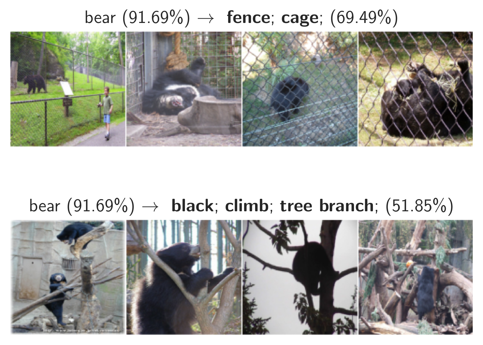
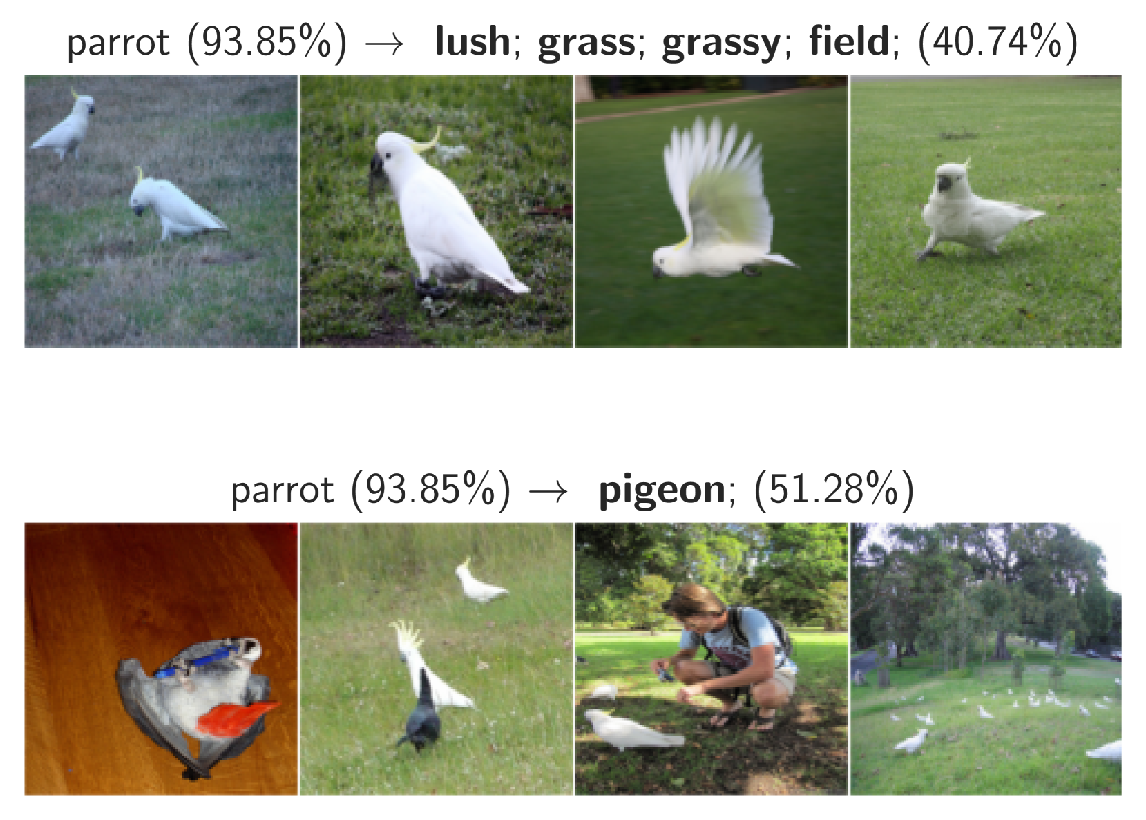
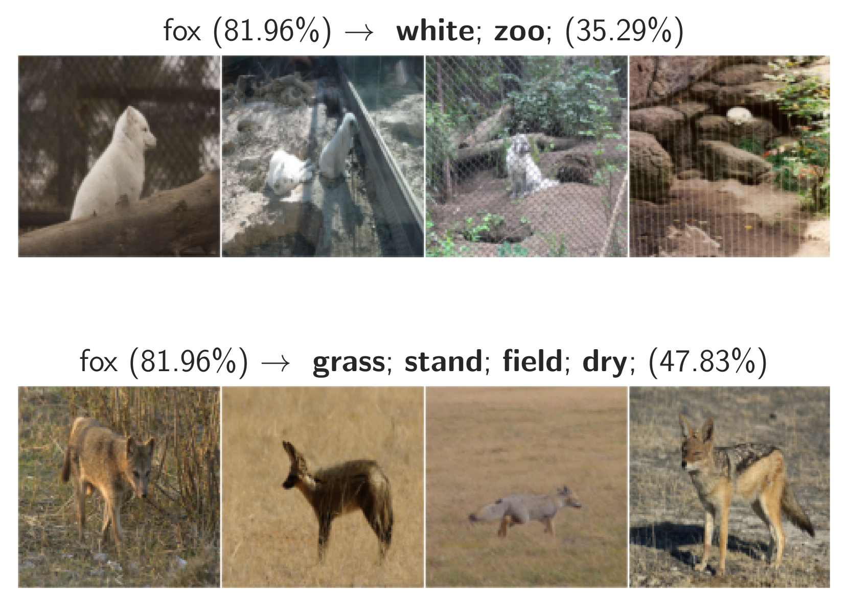
Figure 6: Some visualization of detected failure modes on Living17.

Figure 7: Some visualization of detected failure modes on ImageNet.

Figure 8: Some visualization of detected failure modes on Waterbirds.

A.5 Running the method using different values of (s,a)𝑠 𝑎(s,a)( italic_s , italic_a )

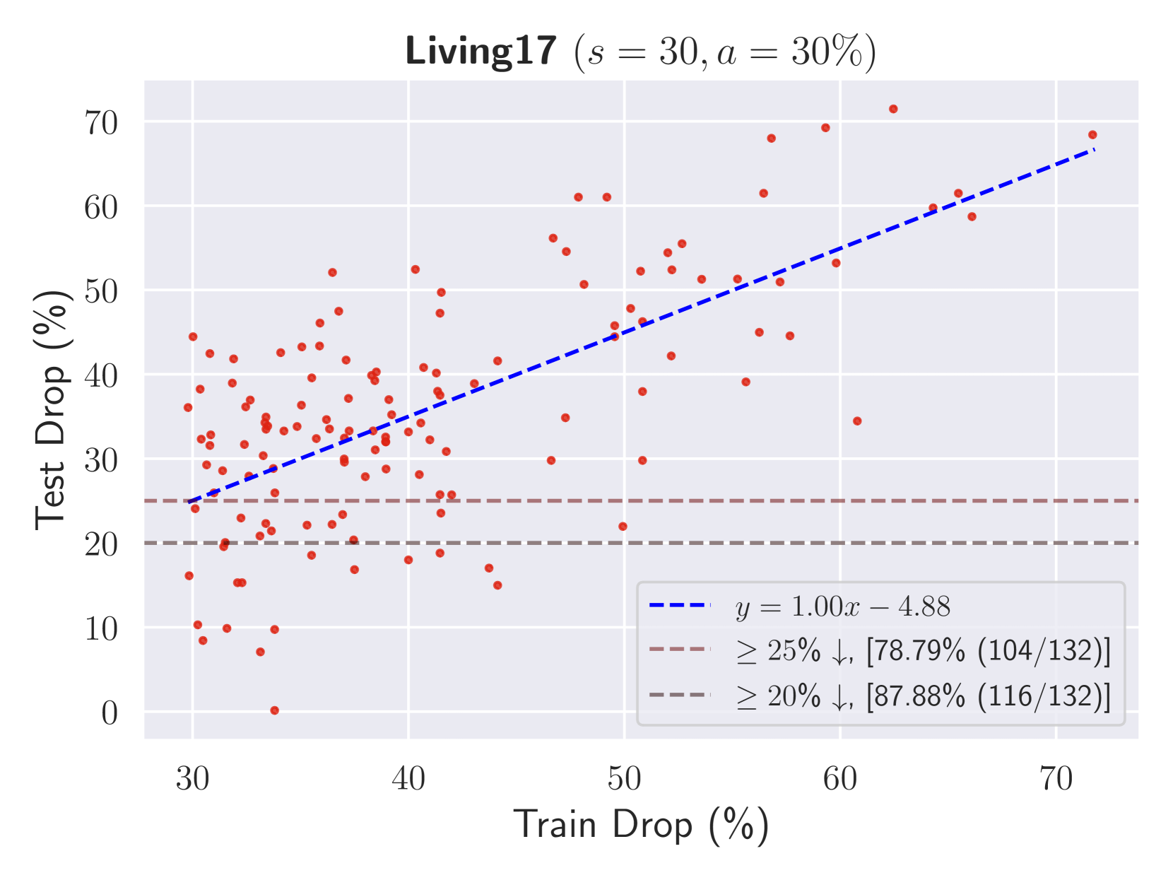
Figure 9: Evaluating detected failure modes on unseen data. (Left): we extract failure modes on Living17 dataset using s=30 𝑠 30 s=30 italic_s = 30 and a=30%𝑎 percent 30 a=30%italic_a = 30 %. 132 132 132 132 failure groups (over 17 17 17 17 classes) are detected and it is observed that around 86.01%percent 86.01 86.01%86.01 % of detected failure modes exhibit at least 25%percent 25 25%25 % drop in accuracy over unseen data that shows a significant degree of generalization. (Right): same results for CelebA dataset where the parameters for failure mode detection is s=50 𝑠 50 s=50 italic_s = 50 and a=30%𝑎 percent 30 a=30%italic_a = 30 %. Around 79.31%percent 79.31 79.31%79.31 % of failure modes show the drop of at least 20%percent 20 20%20 %. The trend of y=x 𝑦 𝑥 y=x italic_y = italic_x is seen in these plots.

In this section, we inspect the effect of different hyperparameters (s,a)𝑠 𝑎(s,a)( italic_s , italic_a ) on the result of our method. By increasing a 𝑎 a italic_a, we aim to detect harder subpopulations, thus, the number of detected failure modes will decrease. By increasing s 𝑠 s italic_s, we detect a group of images associated with a set of tags as a failure mode, if there are a significant number of images within that group. This brings more generalization over detected failure modes while a fewer number of them will be detected by the method. Figure10 shows the generalization plot over different datasets with respect to different hyperparameters.

In Table4, we also report correlation coefficien between train drop and test drop of failure modes over different datasets and values of s 𝑠 s italic_s and a 𝑎 a italic_a.

Table 4: Correlation coefficien between train drop and test drop.

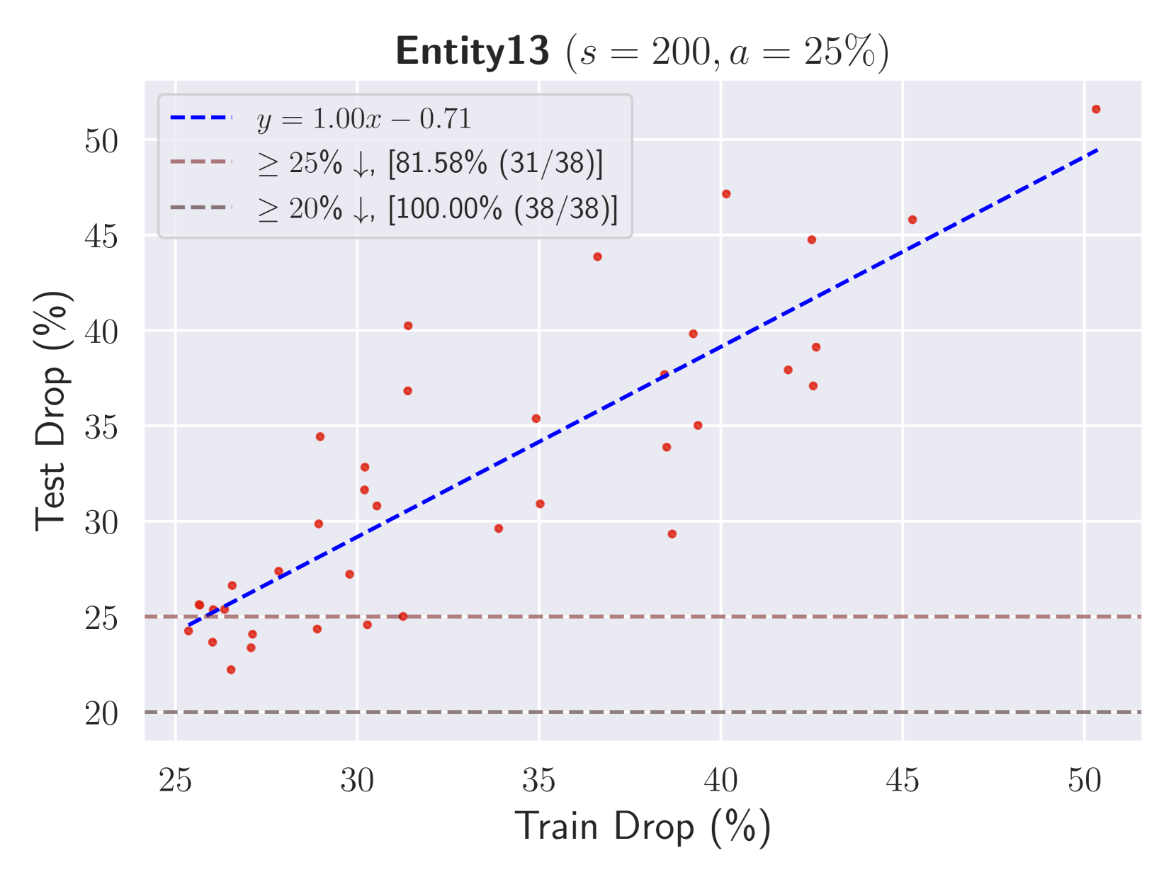
Figure 10: Evaluating detected failure modes on unseen (test) dataset. We extract failure modes on different datasets using different values of (s,a)𝑠 𝑎(s,a)( italic_s , italic_a ).

A.6 Greedy Search

We note that in our experiments, exhaustive search was efficient enough so that we do not need to consider any other approaches. We used some heuristic approaches to improve the efficiency of exhaustive search such as eliminating combination of tags that a few images represent them, etc. However, we developed another greedy search algorithm where at each stage, we pick top tags that condition on them, significantly dropping model accuracy. By running this approach, the space of different choices shrinks and the algorithm becomes faster while missing some of the failure modes.

A.7 DOMINO’s output descriptions

To compare the results of DOMINO with PRIME, we picked DOMINO’s hyperparameters in a way that generates relatively the same number of failure modes. Some of the outputs on Living17 dataset are as follows:

class “salamander”:

*   –a photo of the bullet wound. 
*   –a photo of a lizard. 
*   –a photo of trout fishing. 
*   –a photo of a frog. 
*   –a photo of a hippo. 
*   –a photo of the ventral fin. 
*   –…

class “fox”:

*   –a photo of a gorillas. 
*   –a photo of the titanic sinking. 
*   –a photo of the tract. 
*   –a photo of a coyote. 
*   –a photo of oil shale. 
*   –a photo of the desert. 
*   –a photo of the antarctic. 
*   –a photo of the arctic. 
*   –…

class “cat”:

*   –a photo of the zoological garden. 
*   –a photo of stray dogs. 
*   –a photo of two dogs. 
*   –a photo of the gardener. 
*   –a photo of the tehsil leader. 
*   –…

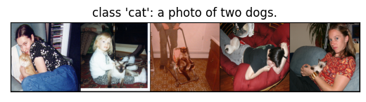
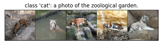
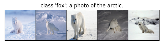
Figure 11: Some of the detected failure modes along with descriptions using DOMINO.

Figure11 shows some visualization of these failure modes. Lack of coherency among images in some of the groups as well as low-quality descriptions can be seen in detected failure modes.

A.8 Quality of Description

We note that failure modes detected by PRIME and DOMINO might be different. However, our metrics only evaluate how well failure modes are described with their corresponding captions and do not consider what images are assigned as failure modes. This enables us to compare different methods with each other. Notably, hyperparameters of different methods play a role in the number of failure modes that a method detects. In order to ensure a fair comparison, we carefully set the hyperparameters for both of methods to yield a similar number of detected failure modes.

Furthermore, it is worth noting that as the similarity score is normalized, comparing this score over different failure modes and different methods is possible. This is why we aggregate similarity score, standard deviation, auroc over all failure modes.

A.9 DOMINO’s generalization

To compare our results with DOMINO (Eyuboglu et al., 2022), we note that this method also outputs some groups as well as descriptions for them. For a failure mode I j subscript 𝐼 𝑗 I_{j}italic_I start_POSTSUBSCRIPT italic_j end_POSTSUBSCRIPT with T j subscript 𝑇 𝑗 T_{j}italic_T start_POSTSUBSCRIPT italic_j end_POSTSUBSCRIPT as its description, we use the same vision-language model that DOMINO uses to collect highly similar images to caption T j subscript 𝑇 𝑗 T_{j}italic_T start_POSTSUBSCRIPT italic_j end_POSTSUBSCRIPT in 𝒟′superscript 𝒟′\mathcal{D^{\prime}}caligraphic_D start_POSTSUPERSCRIPT ′ end_POSTSUPERSCRIPT and obtain I j′subscript superscript 𝐼′𝑗 I^{\prime}{j}italic_I start_POSTSUPERSCRIPT ′ end_POSTSUPERSCRIPT start_POSTSUBSCRIPT italic_j end_POSTSUBSCRIPT. We then evaluate model’s accuracy on images of I j′subscript superscript 𝐼′𝑗 I^{\prime}{j}italic_I start_POSTSUPERSCRIPT ′ end_POSTSUPERSCRIPT start_POSTSUBSCRIPT italic_j end_POSTSUBSCRIPT and expect a hard subpopulation, it should be as hard as I j subscript 𝐼 𝑗 I_{j}italic_I start_POSTSUBSCRIPT italic_j end_POSTSUBSCRIPT. Figure12 shows the generalization of this method. We see a lower degree of generalization in this approach than our method. We observe that generated captions cannot fully describe as hard subpopulations as subpopulations detected on 𝒟 𝒟\mathcal{D}caligraphic_D.

We note that the other method (Jain et al., 2022), only detects a single failure mode for each class in the input and reports around 10 10 10 10 images for that, thus, comparing this method with DOMINO and ours is a bit unfair as those methods detect multiple failure modes with significantly more coverage.

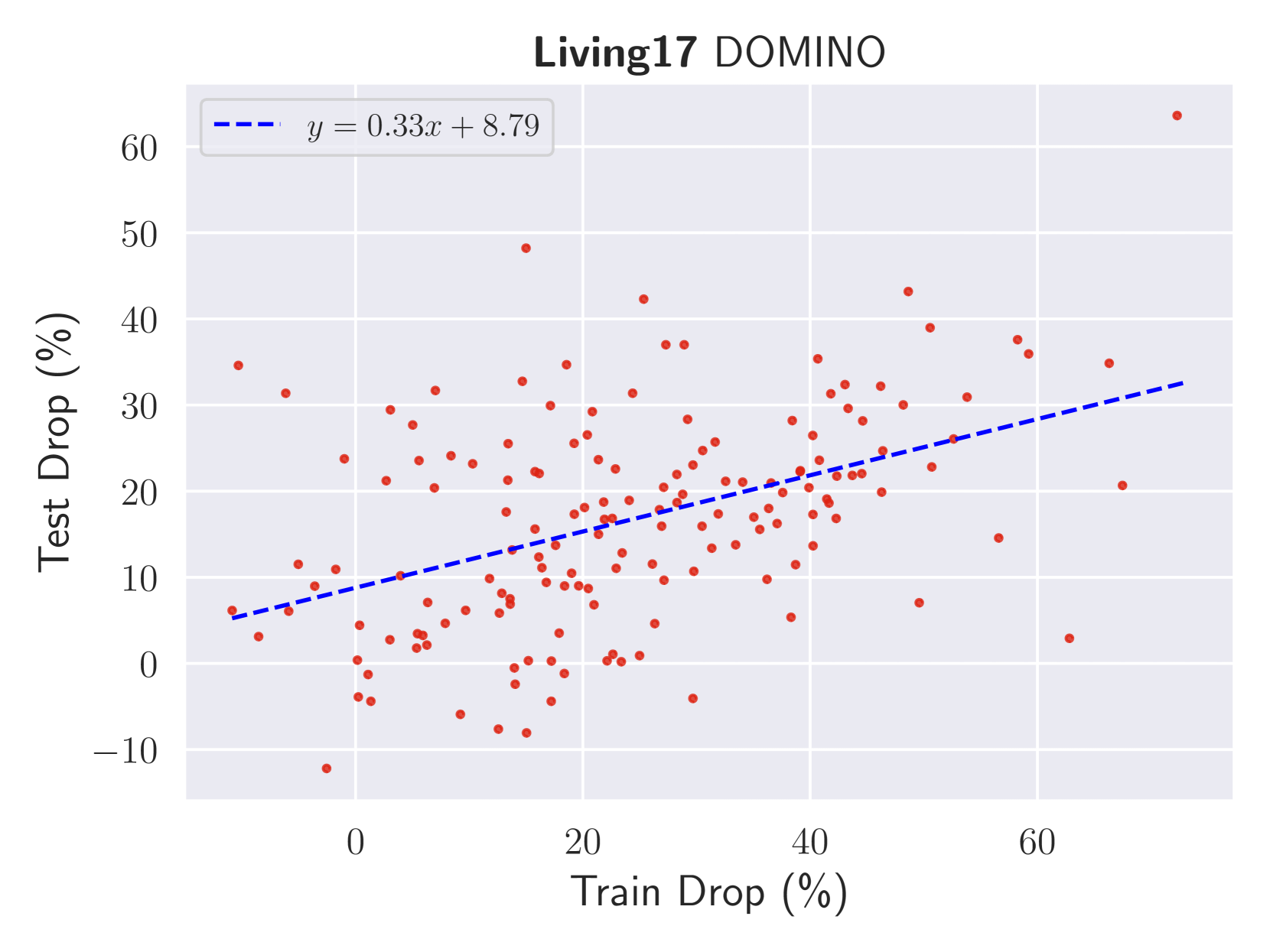
Figure 12: Evaluating detected failure modes by DOMINO on unseen (test) dataset.

A.10 Image Generation

In this section, we elaborate more on the way we generate hard and easy images. To detect easy subpopulations, we randomly pick 2 2 2 2 subset of tags in a way that the model’s accuracy on images representing those tags is 100%percent 100 100%100 %. For the failure modes, we randomly pick two of the detected failure modes in a way that those two groups do not share any common images. It is worth noting that for classes “butterfly” and “dog” we don’t report any results as model’s accuracy for these classes is almost 100%percent 100 100%100 %. Figure13 shows the accuracy gap for different classes.

Here we provide some of the failure/success modes we took and corresponding descriptions used for generative models.

class: “bear”

*   –gray + water →→\rightarrow→ “a photo of a gray bear in water”; 
*   –river →→\rightarrow→ “a photo of a bear in the river” 
*   –cub + climbing + tree →→\rightarrow→ “a photo of a bear cub climbing a tree”; 
*   –black + cub + branch →→\rightarrow→ “a photo of a black bear cub on a tree branch”;

class: “ape”

*   –black + branch →→\rightarrow→ “a photo of a black ape on a tree branch”; 
*   –sky →→\rightarrow→ “a photo of an ape in the sky”; 
*   –gorilla + trunk + sitting →→\rightarrow→ “a photo of a gorilla ape sitting near a tree trunk”; 
*   –mother →→\rightarrow→ “a photo of a mother ape”;

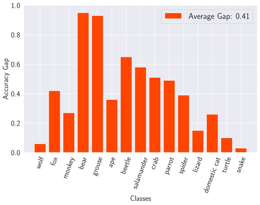
Figure 13: The difference in classifier accuracy between images generated from success mode and failure mode captions on Living17.

A.11 Jain et al. Quality of description

We note that Jain et al. (2022) detects 10 10 10 10 hard and 10 10 10 10 easy images for each class in the dataset and assigns a description to them. However, the way this method generates captions needs humans in the loop as they use a bunch of dataset-oriented words (tokens) that explain different variants of semantic attributes in the dataset. Hence, their method is not scalable to run on many different datasets so we only considered that on Living17 and CelebA. When datasets become larger and more complex, there will exist several failure modes, and Jain et al. (2022) that only extracts a single direction cannot cover many of the failure inputs. Figure14 shows the results on different datasets. We note that on CelebA, they use a very detailed and manually collected set of tokens to generate outputs. However, even in that dataset, their performance is slightly better than ours.

Figure 14: Comparison of the quality of description in our method and Jain et al. (2022). AUROC, Mean, and Standard over different datasets are reported.

A.12 Number of Tags in the Descriptions

In Table5, we bring a more detailed version of Table2 that includes some sampled images of detected failure modes.

Table 5: Accuracy on unseen (test) images for class ape when given tags appear in the inputs. More detailed descriptions not only bring more accurate explanation of images but also can lead to harder example where model’s performance drops more severly. Some randomly sampled images within each group is visualized.

A.13 CUB-200 and CelebA

Table 6: Average number of tags appear in at least α⁢N 𝛼 𝑁\alpha N italic_α italic_N images among N 𝑁 N italic_N closest images to a randomly sampled image in the representation space as well as average number of shared tags in semantic space (CelebA Dataset).

In this section, we show the results reported in Section5.2 over CUB-200 dataset. Table8 includes the results of shared tags in the proximity of images and Table7 includes the statistics of distance between two images in the latent space.

Table 7: Statistics of the distance between two points in CUB-200 dataset conditioned on number of shared tags. Distances are reported using CLIP ViT-B/16 representation space.

Table 8: Average number of tags appear in at least α⁢N 𝛼 𝑁\alpha N italic_α italic_N images among N 𝑁 N italic_N closest images to a randomly sampled image in the representation space as well as average number of shared tags in semantic space (CUB-200 Dataset).

A.14 RAM evaluation on Living17

we run a small-scale human validation study on Living17 (one of the main datasets we used in our paper) to evaluate the accuracy of RAM. We first obtain all tags of class “butterfly” in Living17 and filter out low-frequency tags as discussed in 3.1. 55 55 55 55 tags are remained, i.e.,

T butterfly={black,purple,red,flower,leaf,sit,land,gravel,stone,mud,wildflower,sky,grass,…}.subscript 𝑇 butterfly black purple red flower leaf sit land gravel stone mud wildflower sky grass…T_{\text{butterfly}}={\text{black},\text{purple},\text{red},\text{flower},% \text{leaf},\text{sit},\text{land},\text{gravel},\text{stone},\text{mud},\text% {wildflower},\text{sky},\text{grass},...}.italic_T start_POSTSUBSCRIPT butterfly end_POSTSUBSCRIPT = { black , purple , red , flower , leaf , sit , land , gravel , stone , mud , wildflower , sky , grass , … } .

We take 100 100 100 100 random images from the class “butterfly” in Living17 and evaluate precision/recall of tagging model on those images over tags of T butterfly subscript 𝑇 butterfly T_{\text{butterfly}}italic_T start_POSTSUBSCRIPT butterfly end_POSTSUBSCRIPT. Average Precision of RAM over those 100 100 100 100 images is 86.85%percent 86.85 86.85%86.85 % and average recall is 81.85%percent 81.85 81.85%81.85 %. This shows that RAM is accurate in detection of tags in T butterfly subscript 𝑇 butterfly T_{\text{butterfly}}italic_T start_POSTSUBSCRIPT butterfly end_POSTSUBSCRIPT. It is worth noting that T butterfly subscript 𝑇 butterfly T_{\text{butterfly}}italic_T start_POSTSUBSCRIPT butterfly end_POSTSUBSCRIPT includes a wide range of different objects and attributes, covering a wide range of concepts in those images.

A.15 PRIME hyperparameters

In this section, we elaborate more on each of the hyperparameters in our work. We note that all of the PRIME’s hyperparameters have intuitive definitions, enabling a user to calibrate PRIME toward their specific preferences.

•Parameter a 𝑎 a italic_a controls a trade-off between the difficulty and the quantity of detected failure modes. For example, selecting a high value of a 𝑎 a italic_a results in failure modes that are more difficult but fewer in number. Figure10 shows this trade-off.
•Parameter s 𝑠 s italic_s determines the minimum number of required images inside a group to be detected as a failure mode. Small groups may not be reliable, thus, we filter them out. Larger value for s 𝑠 s italic_s results in more reliable and generalizable failure modes. The choice of s 𝑠 s italic_s also depends on the number of samples within the dataset. For larger datasets, we can assume that different subpopulations are sufficiently represented in the dataset, thus, a larger value for s 𝑠 s italic_s can be used. We refer to Figure10 for observing the effect of s 𝑠 s italic_s.
•l 𝑙 l italic_l determines the maximum number of tags we consider for combination. In datasets we considered, a combination of more than 5 5 5 5 tags would not result in groups with at least s 𝑠 s italic_s images, thus, we set l≤4 𝑙 4 l\leq 4 italic_l ≤ 4 in our experiments. The choice of l 𝑙 l italic_l depends on the dataset and tagging model.
•b i subscript 𝑏 𝑖 b_{i}italic_b start_POSTSUBSCRIPT italic_i end_POSTSUBSCRIPT refers to the degree of necessity for tags inside the failure modes. The current choice of b i subscript 𝑏 𝑖 b_{i}italic_b start_POSTSUBSCRIPT italic_i end_POSTSUBSCRIPT s is only a sample choice, requiring the appearance of each tag to have a significant impact on the difficulty of detected failure modes. One can adjust these hyperparameters based on their preference.

Xet Storage Details

Size:: 103 kB
Xet hash:: 825a61865985a86afa9a72a69f5778146bc071dacd4897309687f7a8b6c3859c

Xet efficiently stores files, intelligently splitting them into unique chunks and accelerating uploads and downloads. More info.