2312/2312.00093.md

Title: GraphDreamer: Compositional 3D Scene Synthesis from Scene Graphs

URL Source: https://arxiv.org/html/2312.00093

Published Time: Wed, 12 Jun 2024 00:08:13 GMT

Markdown Content: \doparttoc\faketableofcontents

Gege Gao 1,2,3,4 Weiyang Liu 1,5,*Anpei Chen 2,3,4 Andreas Geiger 3,4,†Bernhard Schölkopf 1,2,4,†

1 Max Planck Institute for Intelligent Systems – Tübingen 2 ETH Zürich 3 University of Tübingen

4 Tübingen AI Center 5 University of Cambridge*Directional lead†Shared last author

Abstract

As pretrained text-to-image diffusion models become increasingly powerful, recent efforts have been made to distill knowledge from these text-to-image pretrained models for optimizing a text-guided 3D model. Most of the existing methods generate a holistic 3D model from a plain text input. This can be problematic when the text describes a complex scene with multiple objects, because the vectorized text embeddings are inherently unable to capture a complex description with multiple entities and relationships. Holistic 3D modeling of the entire scene further prevents accurate grounding of text entities and concepts. To address this limitation, we propose GraphDreamer, a novel framework to generate compositional 3D scenes from scene graphs, where objects are represented as nodes and their interactions as edges. By exploiting node and edge information in scene graphs, our method makes better use of the pretrained text-to-image diffusion model and is able to fully disentangle different objects without image-level supervision. To facilitate modeling of object-wise relationships, we use signed distance fields as representation and impose a constraint to avoid inter-penetration of objects. To avoid manual scene graph creation, we design a text prompt for ChatGPT to generate scene graphs based on text inputs. We conduct both qualitative and quantitative experiments to validate the effectiveness of GraphDreamer in generating high-fidelity compositional 3D scenes with disentangled object entities.

Figure 1: GraphDreamer takes a scene graph as input and generates a compositional 3D scene where each object is fully disentangled. To save the effort of building a scene graph from scratch, the scene graph can be generated by a language model (e.g., ChatGPT) from a user text input (left box).

1 Introduction

Recent years have witnessed substantial progresses in text-to-3D generation[29, 39, 21], largely due to the rapid development made in text-to-image models[32, 33] and text-image embeddings[31]. This emerging field has attracted considerable attention due to its significant potential to revolutionize the way artists and designers work.

The central idea of current text-to-3D pipelines is to leverage knowledge of a large pretrained text-to-image generative model to optimize each randomly sampled 2D view of a 3D object such that these views resemble what the input text describes. The 3D consistency of these 2D views is typically guaranteed by a proper 3D representation (e.g. missing, neural radiance fields (NeRF)[23] in DreamFusion[29]). Despite being popular, current text-to-3D pipelines still suffer from attribute confusion and guidance collapse. Attribute confusion is a fundamental problem caused by text-image embeddings (e.g. missing, CLIP[31]). For example, models often fail at distinguishing the difference between “a black cat on a pink carpet” and “a pink cat on a black carpet”. This problem may prevent current text-to-3D generation methods from accurately grounding all attributes to corresponding objects. As the text prompt becomes even more complex, involving multiple objects, attribute confusion becomes more significant. Guidance collapse refers to the cases where the text prompt is (partially) ignored or misinterpreted by the model. This typically also happens as the text prompt gets more complex. For example, “a teddy bear pushing a shopping cart and holding baloons”, with “teddy bear” being ignored. These problems largely limit the practical utility of text-to-3D generation techniques.

A straightforward solution is to model the multi-object 3D scene in a compositional way. Following this insight, recent methods [18, 28, 5, 47] condition on additional context information such as 3D layout which provides the size and location of each object in the form of non-overlapping 3D bounding boxes. While a non-overlapping 3D layout can certainly help to produce a compositional 3D scene with each object present, it injects a strong prior and greatly limits the diversity of generated scenes. The non-overlapping 3D box assumption can easily break when objects are irregular (non-cubic) and obscuring each other. For example, the text prompt “an astronaut riding a horse” can not be represented by two non-overlapping bounding boxes. To avoid these limitations while still achieving object decomposition, we propose GraphDreamer, which takes a scene graph (e.g. missing, [13]) as input and generates a compositional 3D scene. Unlike 3D bounding boxes, scene graphs are spatially more relaxed and can model complex object interaction. While scene graphs are generally easier to specify than spatial 3D layouts, we also design a text prompt to query ChatGPT that enables the automatic generation of a scene graph from unstructured text. See Figure1 for an illustrative example.

GraphDreamer is guided by the insight that a scene graph can be decomposed into a separate and semantically unambiguous text description of every node and edge 1 1 1 Cf.the assumption of independent causal mechanisms[34]. The decomposition of a scene graph into multiple textual descriptions makes it possible to distill knowledge from text-to-image diffusion models, similar to common text-to-3D methods. Specifically, to allow each object to be disentangled from the other objects in the scene, we use separate identity-aware positional encoder networks (i.e. missing, object feature fields) to encode object-level semantic information and a shared Signed Distance Field(SDF) network to decode the SDF value from identity-aware positional features. The color value is decoded in a way similar to the SDF value. Scene-level rendering is performed by integrating objects based on the smallest SDF value at each sampled point in 3D space. More importantly, with both SDF and color values of each object, we propose an identity-aware object rendering that, in addition to a global rendering of the entire 3D scene, renders different objects separately. Our local identity-aware rendering allows the gradient from the text-dependent distillation loss (e.g. missing, score distillation sampling[29]) to be back-propagated selectively to corresponding objects without affecting the other objects. The overall 3D scene will be simultaneously optimized with the global text description to match the scene semantics to the global text. In summary, we make the following contributions:

• •To the best of our knowledge, GraphDreamer is the first 3D generation method that can synthesize compositional 3D scenes from either scene graphs or unstructured text descriptions. No 3D bounding boxes are required as input.
• •GraphDreamer uses scene graphs to construct a disentangled representation where each object is optimized via its related text description, avoiding object-level ambiguity.
• •GraphDreamer is able to produce high-fidelity complex 3D scenes with disentangled objects, outperforming both state-of-the-art text-to-3D methods and existing 3D-bounding-box-based compositional text-to-3D methods.
• •In AppendixC, we envision a new paradigm of semantic 3D reconstruction – Inverse Semantics, where a vision-language model (e.g. missing, GPT4-V) is used to extract a scene graph from an input image (i.e. missing, scene graph encoder) and GraphDreamer is used to generate a compositional 3D scene from the scene graph (i.e. missing, scene graph decoder).

2 Related Work

Text-to-2D generation. Driven by large-scale image-text aligned datasets[35], text-to-image generation models[1, 33, 32] have made great progress in producing highly realistic images. Among these models, generative diffusion models learn to gradually transform a noisy latent z 𝑧 z italic_z with noise ϵ italic-ϵ\epsilon italic_ϵ typically from a Gaussian distribution, towards image data x 𝑥 x italic_x that reproduce the semantics of a given text prompt y 𝑦 y italic_y. This generative process slowly adds structure to the noise, based on a weighted denoising score matching objective [27, 12].

2D-lifting for 3D generation. In contrast to existing text-to-image generation models, text-guided 3D generative models[10, 24, 29, 39, 21, 38, 22, 26] usually optimize a 3D model by guiding its randomly rendered 2D view based on the pretraining knowledge of some text-to-image generation model, because of the shortage of text-3D paired assets. DreamFusion[29] and subsequent work[17, 42, 4, 44, 37] propose to optimize the 3D model by distilling a pretrained diffusion model[33, 32] via score distillation sampling[39].

Generate objects with SDF. In text-to-3D generation, recent works[10, 29, 40, 17, 42, 39, 19, 21, 37] parameterized the 3D scene as a NeRF[23, 2] or a hybrid pipeline combining NeRFs with a mesh refiner[11, 17, 36, 38]. In our approach, we use a signed distance field (SDF) as the geometry representation instead of NeRF densities, as we aim at modeling multi-object scenes in a compositional way, where objects may be coupled in various ways. SDF provides crucial inside/outside information, allowing for geometry constraints to prevent unexpected intersections between objects, and is ideal for complex scenes as it facilitates customization of initial locations and scales of object SDFs.

Hybrid 3D representation for disentanglement. Another line of work uses hybrid representations to learn disentangled 3D objects[15, 43, 20]. The works [6, 7] put forward a hybrid approach that represents the face/body as meshes and the hair/clothing as NeRFs, enabling a disentangled reconstruction of avatars. [48] adopts this representation and proposes a text-to-3D method that generates compositional head avatars. However, the use of a parametric head model limits this method to human head generation. Their disentanglement only applies to two objects (e.g. missing, face and hair), and in contrast, ours can be used for multiple objects.

3 Preliminaries

Score distillation sampling (SDS). SDS[29] is a technique that optimizes a 3D model by distilling a pretrained text-to-image diffusion model. Given a noisy image z t subscript 𝑧 𝑡 z_{t}italic_z start_POSTSUBSCRIPT italic_t end_POSTSUBSCRIPT rendered from a 3D model parameterized by Θ Θ\Theta roman_Θ, and a pretrained text-to-image diffusion model with a learned noise prediction network ϵ ϕ⁢(⋅)subscript italic-ϵ italic-ϕ⋅\epsilon_{\phi}(\cdot)italic_ϵ start_POSTSUBSCRIPT italic_ϕ end_POSTSUBSCRIPT ( ⋅ ), SDS uses ϵ ϕ⁢(⋅)subscript italic-ϵ italic-ϕ⋅\epsilon_{\phi}(\cdot)italic_ϵ start_POSTSUBSCRIPT italic_ϕ end_POSTSUBSCRIPT ( ⋅ ) as a score function that predicts the sampled noise ϵ italic-ϵ\epsilon italic_ϵ contained in x t subscript 𝑥 𝑡 x_{t}italic_x start_POSTSUBSCRIPT italic_t end_POSTSUBSCRIPT at noise level t 𝑡 t italic_t as ϵ^ϕ⁢(y,t)=ϵ ϕ⁢(z t;y,t)subscript^italic-ϵ italic-ϕ 𝑦 𝑡 subscript italic-ϵ italic-ϕ subscript 𝑧 𝑡 𝑦 𝑡\hat{\epsilon}{\phi}(y,t)=\epsilon{\phi}(z_{t};y,t)over^ start_ARG italic_ϵ end_ARG start_POSTSUBSCRIPT italic_ϕ end_POSTSUBSCRIPT ( italic_y , italic_t ) = italic_ϵ start_POSTSUBSCRIPT italic_ϕ end_POSTSUBSCRIPT ( italic_z start_POSTSUBSCRIPT italic_t end_POSTSUBSCRIPT ; italic_y , italic_t ), where y 𝑦 y italic_y is a given conditional text embedding. The score is then used to warp the noisy z t subscript 𝑧 𝑡 z_{t}italic_z start_POSTSUBSCRIPT italic_t end_POSTSUBSCRIPT towards real image distributions, by guiding the direction of the gradients that update the parameters Θ Θ\Theta roman_Θ of the 3D model:

∇Θ ℒ⁢(z;y)=𝔼 t,ϵ⁢[w⁢(t)⁢(ϵ^ϕ⁢(y,t)−ϵ)⁢∂z∂Θ]subscript∇Θ ℒ 𝑧 𝑦 subscript 𝔼 𝑡 italic-ϵ delimited-[]𝑤 𝑡 subscript^italic-ϵ italic-ϕ 𝑦 𝑡 italic-ϵ 𝑧 Θ\nabla_{\Theta}\mathcal{L}(z;y)=\mathbb{E}{t,\epsilon}\biggl{[}w(t)\Bigl{(}% \hat{\epsilon}{\phi}(y,t)-\epsilon\Bigr{)}\frac{\partial z}{\partial\Theta}% \biggr{]}∇ start_POSTSUBSCRIPT roman_Θ end_POSTSUBSCRIPT caligraphic_L ( italic_z ; italic_y ) = blackboard_E start_POSTSUBSCRIPT italic_t , italic_ϵ end_POSTSUBSCRIPT italic_w ( italic_t ) ( over^ start_ARG italic_ϵ end_ARG start_POSTSUBSCRIPT italic_ϕ end_POSTSUBSCRIPT ( italic_y , italic_t ) - italic_ϵ ) divide start_ARG ∂ italic_z end_ARG start_ARG ∂ roman_Θ end_ARG

where w⁢(t)𝑤 𝑡 w(t)italic_w ( italic_t ) is a weighting function that depends on t 𝑡 t italic_t and ϵ italic-ϵ\epsilon italic_ϵ is the sampled isotropic Gaussian noise, ϵ∼𝒩⁢(𝟎,𝐈)similar-to italic-ϵ 𝒩 0 𝐈\epsilon\sim\mathcal{N}(\mathbf{0},\mathbf{I})italic_ϵ ∼ caligraphic_N ( bold_0 , bold_I ).

SDF volume rendering. To render a pixel color of a target camera, we cast a ray 𝐫 𝐫\mathbf{r}bold_r from the camera center 𝐨 𝐨\mathbf{o}bold_o along its viewing direction 𝐝 𝐝\mathbf{d}bold_d, then sample a series of points 𝐩=𝐨+t⁢𝐝 𝐩 𝐨 𝑡 𝐝\mathbf{p}=\mathbf{o}+t\mathbf{d}bold_p = bold_o + italic_t bold_d in between the near and far intervals [t n,t f]subscript 𝑡 𝑛 subscript 𝑡 𝑓[t_{n},t_{f}][ italic_t start_POSTSUBSCRIPT italic_n end_POSTSUBSCRIPT , italic_t start_POSTSUBSCRIPT italic_f end_POSTSUBSCRIPT ]. Following NeRF[23], the ray color C⁢(𝐫)𝐶 𝐫 C(\mathbf{r})italic_C ( bold_r ) can be approximated by integrating the point samples,

C⁢(𝐫)=∑i=1 N w i⁢c i=∑i=1 N T i⁢α i⁢c i 𝐶 𝐫 superscript subscript 𝑖 1 𝑁 subscript 𝑤 𝑖 subscript 𝑐 𝑖 superscript subscript 𝑖 1 𝑁 subscript 𝑇 𝑖 subscript 𝛼 𝑖 subscript 𝑐 𝑖 C(\mathbf{r})=\sum_{i=1}^{N}w_{i}c_{i}=\sum_{i=1}^{N}T_{i}\alpha_{i}c_{i}italic_C ( bold_r ) = ∑ start_POSTSUBSCRIPT italic_i = 1 end_POSTSUBSCRIPT start_POSTSUPERSCRIPT italic_N end_POSTSUPERSCRIPT italic_w start_POSTSUBSCRIPT italic_i end_POSTSUBSCRIPT italic_c start_POSTSUBSCRIPT italic_i end_POSTSUBSCRIPT = ∑ start_POSTSUBSCRIPT italic_i = 1 end_POSTSUBSCRIPT start_POSTSUPERSCRIPT italic_N end_POSTSUPERSCRIPT italic_T start_POSTSUBSCRIPT italic_i end_POSTSUBSCRIPT italic_α start_POSTSUBSCRIPT italic_i end_POSTSUBSCRIPT italic_c start_POSTSUBSCRIPT italic_i end_POSTSUBSCRIPT(2)

where w i subscript 𝑤 𝑖 w_{i}italic_w start_POSTSUBSCRIPT italic_i end_POSTSUBSCRIPT is the color weighting function, T i subscript 𝑇 𝑖 T_{i}italic_T start_POSTSUBSCRIPT italic_i end_POSTSUBSCRIPT represents the cumulative transmittance, which is calculated as T i=∏j=1 i−1(1−α j)subscript 𝑇 𝑖 superscript subscript product 𝑗 1 𝑖 1 1 subscript 𝛼 𝑗 T_{i}=\prod_{j=1}^{i-1}(1-\alpha_{j})italic_T start_POSTSUBSCRIPT italic_i end_POSTSUBSCRIPT = ∏ start_POSTSUBSCRIPT italic_j = 1 end_POSTSUBSCRIPT start_POSTSUPERSCRIPT italic_i - 1 end_POSTSUPERSCRIPT ( 1 - italic_α start_POSTSUBSCRIPT italic_j end_POSTSUBSCRIPT ), and α i subscript 𝛼 𝑖\alpha_{i}italic_α start_POSTSUBSCRIPT italic_i end_POSTSUBSCRIPT denotes the piece-wise constant opacity value for the i 𝑖 i italic_i-th sub-interval, with α i∈[0,1]subscript 𝛼 𝑖 0 1\alpha_{i}\in[0,1]italic_α start_POSTSUBSCRIPT italic_i end_POSTSUBSCRIPT ∈ [ 0 , 1 ].

Unlike NeRFs that directly predict the density for a given position 𝐩 𝐩\mathbf{p}bold_p, methods based on implicit surface representation learn to map 𝐩 𝐩\mathbf{p}bold_p to a signed distance value with a trainable network and extract the density[46] or opacity[41] from the SDF with a deterministic transformation. We extract the opacity following NeuS[41]. NeuS formulates the transformation function based on an unbiased weighting function, which ensures that the pixel color is dominated by the intersection point of camera ray with the zero-level set of SDF,

α i=max⁢(Φ β⁢(u i)−Φ β⁢(u i+1)Φ β⁢(u i),0)subscript 𝛼 𝑖 max subscript Φ 𝛽 subscript 𝑢 𝑖 subscript Φ 𝛽 subscript 𝑢 𝑖 1 subscript Φ 𝛽 subscript 𝑢 𝑖 0\alpha_{i}=\text{max}\left(\frac{\Phi_{\beta}(u_{i})-\Phi_{\beta}(u_{i+1})}{% \Phi_{\beta}(u_{i})},0\right)italic_α start_POSTSUBSCRIPT italic_i end_POSTSUBSCRIPT = max ( divide start_ARG roman_Φ start_POSTSUBSCRIPT italic_β end_POSTSUBSCRIPT ( italic_u start_POSTSUBSCRIPT italic_i end_POSTSUBSCRIPT ) - roman_Φ start_POSTSUBSCRIPT italic_β end_POSTSUBSCRIPT ( italic_u start_POSTSUBSCRIPT italic_i + 1 end_POSTSUBSCRIPT ) end_ARG start_ARG roman_Φ start_POSTSUBSCRIPT italic_β end_POSTSUBSCRIPT ( italic_u start_POSTSUBSCRIPT italic_i end_POSTSUBSCRIPT ) end_ARG , 0 )(3)

where Φ β⁢(⋅)subscript Φ 𝛽⋅\Phi_{\beta}(\cdot)roman_Φ start_POSTSUBSCRIPT italic_β end_POSTSUBSCRIPT ( ⋅ ) is the Sigmoid function with a trainable steepness β 𝛽\beta italic_β, and u i subscript 𝑢 𝑖 u_{i}italic_u start_POSTSUBSCRIPT italic_i end_POSTSUBSCRIPT is the SDF value of the sampled position.

4 Method

Consider generating a scene of M 𝑀 M italic_M objects, 𝒪={o i}i=1 M 𝒪 superscript subscript subscript 𝑜 𝑖 𝑖 1 𝑀\mathcal{O}={o_{i}}_{i=1}^{M}caligraphic_O = { italic_o start_POSTSUBSCRIPT italic_i end_POSTSUBSCRIPT } start_POSTSUBSCRIPT italic_i = 1 end_POSTSUBSCRIPT start_POSTSUPERSCRIPT italic_M end_POSTSUPERSCRIPT from a global text prompt y g superscript 𝑦 𝑔 y^{g}italic_y start_POSTSUPERSCRIPT italic_g end_POSTSUPERSCRIPT. When the scene is complex or has many attributes and inter-object relationships to specify, y g superscript 𝑦 𝑔 y^{g}italic_y start_POSTSUPERSCRIPT italic_g end_POSTSUPERSCRIPT will become very long, and the generation will be accompanied by guidance collapse[3, 16]. We thus propose to first generate a scene graph 𝒢⁢(𝒪)𝒢 𝒪\mathcal{G}(\mathcal{O})caligraphic_G ( caligraphic_O ) from y g superscript 𝑦 𝑔 y^{g}italic_y start_POSTSUPERSCRIPT italic_g end_POSTSUPERSCRIPT following the setting of[13], which precisely describes object attributes and inter-object relationships. We provide an example of a four-object scene in Figure1 for better illustration.

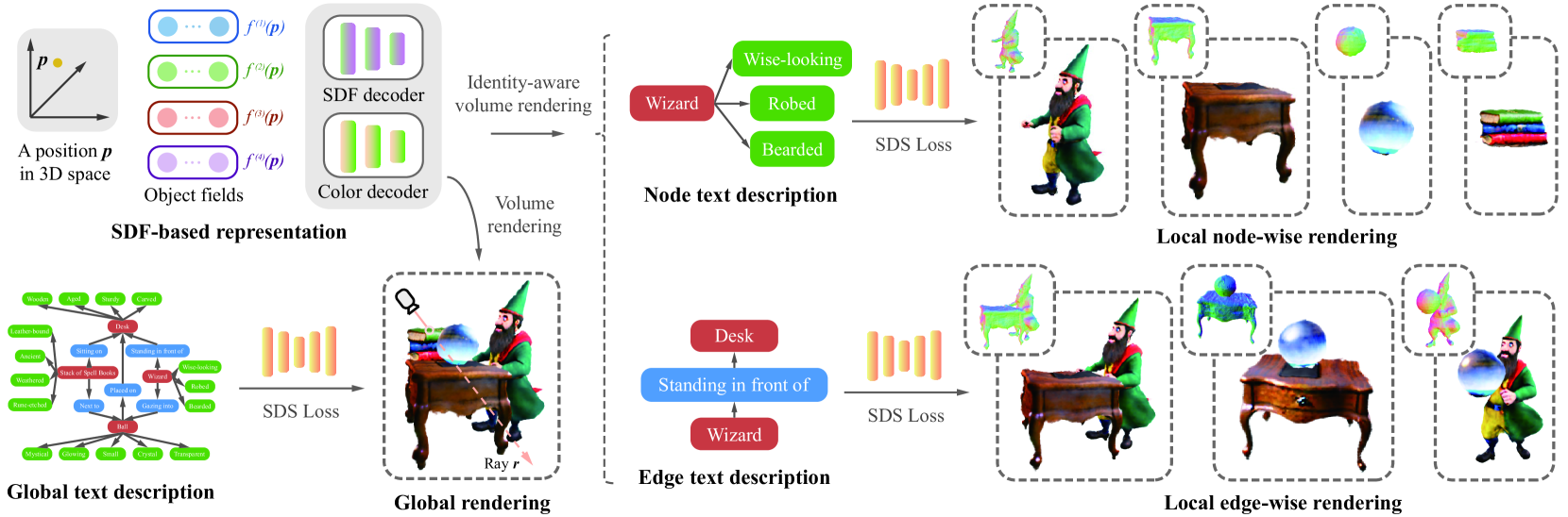
Figure 2: The overall pipeline of GraphDreamer. Specifically, GraphDreamer first decomposes the scene graph into global, node-wise and edge-wise text description, and then optimizes the SDF-based objects in the 3D scene using their corresponding text description.

4.1 Leveraging Scene Graphs for Text Grounding

Given user text input y g superscript 𝑦 𝑔 y^{g}italic_y start_POSTSUPERSCRIPT italic_g end_POSTSUPERSCRIPT, objects {o i}i=1 M superscript subscript subscript 𝑜 𝑖 𝑖 1 𝑀{o_{i}}{i=1}^{M}{ italic_o start_POSTSUBSCRIPT italic_i end_POSTSUBSCRIPT } start_POSTSUBSCRIPT italic_i = 1 end_POSTSUBSCRIPT start_POSTSUPERSCRIPT italic_M end_POSTSUPERSCRIPT in the text (which can be detected either manually or automatically, e.g. missing, using ChatGPT 2 2 2 ChatGPT4, https://chat.openai.com) form the nodes in graph 𝒢⁢(𝒪)𝒢 𝒪\mathcal{G}(\mathcal{O})caligraphic_G ( caligraphic_O ), as shown in Figure1. To provide more details to an object o i subscript 𝑜 𝑖 o{i}italic_o start_POSTSUBSCRIPT italic_i end_POSTSUBSCRIPT, the user can add additional descriptions, such as “Wise-looking” and “Leather-bound”, which become the attributes attached to o i subscript 𝑜 𝑖 o_{i}italic_o start_POSTSUBSCRIPT italic_i end_POSTSUBSCRIPT in 𝒢⁢(𝒪)𝒢 𝒪\mathcal{G}(\mathcal{O})caligraphic_G ( caligraphic_O ). Combining o i subscript 𝑜 𝑖 o_{i}italic_o start_POSTSUBSCRIPT italic_i end_POSTSUBSCRIPT with all its attributes simply by commas, we get an object prompt y(i)superscript 𝑦 𝑖 y^{(i)}italic_y start_POSTSUPERSCRIPT ( italic_i ) end_POSTSUPERSCRIPT for o i subscript 𝑜 𝑖 o_{i}italic_o start_POSTSUBSCRIPT italic_i end_POSTSUBSCRIPT that can be processed by text encoders.

The relationship between each pair of objects o i subscript 𝑜 𝑖 o_{i}italic_o start_POSTSUBSCRIPT italic_i end_POSTSUBSCRIPT and o j subscript 𝑜 𝑗 o_{j}italic_o start_POSTSUBSCRIPT italic_j end_POSTSUBSCRIPT is transformed into edge e i,j subscript 𝑒 𝑖 𝑗 e_{i,j}italic_e start_POSTSUBSCRIPT italic_i , italic_j end_POSTSUBSCRIPT in 𝒢⁢(𝒪)𝒢 𝒪\mathcal{G}(\mathcal{O})caligraphic_G ( caligraphic_O ). For instance, the edge between node “Wizard” and “Desk” is “Standing in front of”. For a graph with M 𝑀 M italic_M nodes, there are possibly C 2 M superscript subscript 𝐶 2 𝑀 C_{2}^{M}italic_C start_POSTSUBSCRIPT 2 end_POSTSUBSCRIPT start_POSTSUPERSCRIPT italic_M end_POSTSUPERSCRIPT edges. By combining o i subscript 𝑜 𝑖 o_{i}italic_o start_POSTSUBSCRIPT italic_i end_POSTSUBSCRIPT, e i,j subscript 𝑒 𝑖 𝑗 e_{i,j}italic_e start_POSTSUBSCRIPT italic_i , italic_j end_POSTSUBSCRIPT, and o j subscript 𝑜 𝑗 o_{j}italic_o start_POSTSUBSCRIPT italic_j end_POSTSUBSCRIPT, we obtain edge prompt y(i,j)superscript 𝑦 𝑖 𝑗 y^{(i,j)}italic_y start_POSTSUPERSCRIPT ( italic_i , italic_j ) end_POSTSUPERSCRIPT that exactly defines the pairwise relationship, e.g. missing, “Wizard standing in front of Wooden Desk”. Note that there might be no edge between two nodes, e.g. missing, between “Wizard” and “Stack of Ancient Spell Books”. We denote the number of existing edges in 𝒢⁢(𝒪)𝒢 𝒪\mathcal{G}(\mathcal{O})caligraphic_G ( caligraphic_O ) as K 𝐾 K italic_K, with K≤C 2 M 𝐾 superscript subscript 𝐶 2 𝑀 K\leq C_{2}^{M}italic_K ≤ italic_C start_POSTSUBSCRIPT 2 end_POSTSUBSCRIPT start_POSTSUPERSCRIPT italic_M end_POSTSUPERSCRIPT.

From this example, we also see that using graph 𝒢⁢(𝒪)𝒢 𝒪\mathcal{G}(\mathcal{O})caligraphic_G ( caligraphic_O ) is a better way to customize a scene compared to a pure text description y g superscript 𝑦 𝑔 y^{g}italic_y start_POSTSUPERSCRIPT italic_g end_POSTSUPERSCRIPT, in terms of both flexibility in attaching attributes to objects and accuracy in defining relationships. By processing the input scene graph, we now obtain a set of (1+M+K)1 𝑀 𝐾(1+M+K)( 1 + italic_M + italic_K ) prompts 𝒴⁢(𝒢⁢(𝒪))𝒴 𝒢 𝒪\mathcal{Y}\bigl{(}\mathcal{G}(\mathcal{O})\bigr{)}caligraphic_Y ( caligraphic_G ( caligraphic_O ) ) as:

𝒴⁢(𝒢⁢(𝒪))={y g,y(i),y(i,j)∣o i∈𝒪,e i,j∈𝒢⁢(𝒪)}𝒴 𝒢 𝒪 conditional-set superscript 𝑦 𝑔 superscript 𝑦 𝑖 superscript 𝑦 𝑖 𝑗 formulae-sequence subscript 𝑜 𝑖 𝒪 subscript 𝑒 𝑖 𝑗 𝒢 𝒪\mathcal{Y}\bigl{(}\mathcal{G}(\mathcal{O})\bigr{)}=\bigl{{}y^{g},y^{(i)},y^{% (i,j)}\mid o_{i}\in\mathcal{O},e_{i,j}\in\mathcal{G}(\mathcal{O})\bigr{}}caligraphic_Y ( caligraphic_G ( caligraphic_O ) ) = { italic_y start_POSTSUPERSCRIPT italic_g end_POSTSUPERSCRIPT , italic_y start_POSTSUPERSCRIPT ( italic_i ) end_POSTSUPERSCRIPT , italic_y start_POSTSUPERSCRIPT ( italic_i , italic_j ) end_POSTSUPERSCRIPT ∣ italic_o start_POSTSUBSCRIPT italic_i end_POSTSUBSCRIPT ∈ caligraphic_O , italic_e start_POSTSUBSCRIPT italic_i , italic_j end_POSTSUBSCRIPT ∈ caligraphic_G ( caligraphic_O ) }(4)

which are used to guide scene generation from the perspective of both individual objects and pairwise relationships.

GraphDreamer consists of three learnable modules: a positional feature encoder ℱ θ⁢(⋅)subscript ℱ 𝜃⋅\mathcal{F}{\theta}(\cdot)caligraphic_F start_POSTSUBSCRIPT italic_θ end_POSTSUBSCRIPT ( ⋅ ), a signed distance network u ϕ 1⁢(⋅)subscript 𝑢 subscript italic-ϕ 1⋅u{\phi_{1}}(\cdot)italic_u start_POSTSUBSCRIPT italic_ϕ start_POSTSUBSCRIPT 1 end_POSTSUBSCRIPT end_POSTSUBSCRIPT ( ⋅ ), and a radiance network c ϕ 2⁢(⋅)subscript 𝑐 subscript italic-ϕ 2⋅c_{\phi_{2}}(\cdot)italic_c start_POSTSUBSCRIPT italic_ϕ start_POSTSUBSCRIPT 2 end_POSTSUBSCRIPT end_POSTSUBSCRIPT ( ⋅ ). The entire model is parameterized by Θ={θ,ϕ 1,ϕ 2}Θ 𝜃 subscript italic-ϕ 1 subscript italic-ϕ 2\Theta={\theta,\phi_{1},\phi_{2}}roman_Θ = { italic_θ , italic_ϕ start_POSTSUBSCRIPT 1 end_POSTSUBSCRIPT , italic_ϕ start_POSTSUBSCRIPT 2 end_POSTSUBSCRIPT }. There are two goals in optimizing GraphDreamer: (i) to model the complete geometry and appearance of each object, and (ii) to ensure that object attributes and interrelationships are in accordance with the scene graph 𝒢⁢(𝒪)𝒢 𝒪\mathcal{G}(\mathcal{O})caligraphic_G ( caligraphic_O ). The overall training process is illustrated in Figure 2.

4.2 Disentangled Modeling of Objects

Positional encodings are useful for networks to identify the location it is currently processing. To achieve the first goal of making objects separable, we need to additionally identify which object a position belongs to. Therefore, instead of one positional feature embedding, we encode a position 𝐩 𝐩\mathbf{p}bold_p into multiple feature embeddings by introducing a set of positional hash feature encoders, each parameterized by θ i subscript 𝜃 𝑖\theta_{i}italic_θ start_POSTSUBSCRIPT italic_i end_POSTSUBSCRIPT, corresponding to the number of objects,

ℱ θ⁢(⋅)={ℱ θ i⁢(⋅)}i=1 M θ={θ i}i=1 M formulae-sequence subscript ℱ 𝜃⋅superscript subscript subscript ℱ subscript 𝜃 𝑖⋅𝑖 1 𝑀 𝜃 superscript subscript subscript 𝜃 𝑖 𝑖 1 𝑀\mathcal{F}{\theta}(\cdot)={\mathcal{F}{\theta_{i}}(\cdot)}{i=1}^{M}{}{% }{}{}~{}\theta={\theta{i}}_{i=1}^{M}caligraphic_F start_POSTSUBSCRIPT italic_θ end_POSTSUBSCRIPT ( ⋅ ) = { caligraphic_F start_POSTSUBSCRIPT italic_θ start_POSTSUBSCRIPT italic_i end_POSTSUBSCRIPT end_POSTSUBSCRIPT ( ⋅ ) } start_POSTSUBSCRIPT italic_i = 1 end_POSTSUBSCRIPT start_POSTSUPERSCRIPT italic_M end_POSTSUPERSCRIPT italic_θ = { italic_θ start_POSTSUBSCRIPT italic_i end_POSTSUBSCRIPT } start_POSTSUBSCRIPT italic_i = 1 end_POSTSUBSCRIPT start_POSTSUPERSCRIPT italic_M end_POSTSUPERSCRIPT(5)

These feature encoders then form different object fields, i.e. missing, one field per object across the same scene space Ω⊂ℝ 3 Ω superscript ℝ 3\Omega\subset\mathbb{R}^{3}roman_Ω ⊂ blackboard_R start_POSTSUPERSCRIPT 3 end_POSTSUPERSCRIPT.

Individualized object fields. Given a position 𝐩∈Ω 𝐩 Ω\mathbf{p}\in\Omega bold_p ∈ roman_Ω, the feature that forms the field of object o i subscript 𝑜 𝑖 o_{i}italic_o start_POSTSUBSCRIPT italic_i end_POSTSUBSCRIPT is obtained as:

f(i)⁢(𝐩)=ℱ θ i⁢(𝐩)∈ℝ F i∈{1,⋯,M}formulae-sequence superscript 𝑓 𝑖 𝐩 subscript ℱ subscript 𝜃 𝑖 𝐩 superscript ℝ 𝐹 𝑖 1⋯𝑀 f^{(i)}(\mathbf{p})=\mathcal{F}{\theta{i}}(\mathbf{p})\in\mathbb{R}^{F}{}{% }{}{}i\in{1,\cdots,M}italic_f start_POSTSUPERSCRIPT ( italic_i ) end_POSTSUPERSCRIPT ( bold_p ) = caligraphic_F start_POSTSUBSCRIPT italic_θ start_POSTSUBSCRIPT italic_i end_POSTSUBSCRIPT end_POSTSUBSCRIPT ( bold_p ) ∈ blackboard_R start_POSTSUPERSCRIPT italic_F end_POSTSUPERSCRIPT italic_i ∈ { 1 , ⋯ , italic_M }(6)

where F 𝐹 F italic_F is the number of feature dimensions, the same for all ℱ θ i⁢(⋅)subscript ℱ subscript 𝜃 𝑖⋅\mathcal{F}{\theta{i}}(\cdot)caligraphic_F start_POSTSUBSCRIPT italic_θ start_POSTSUBSCRIPT italic_i end_POSTSUBSCRIPT end_POSTSUBSCRIPT ( ⋅ ). Here, for each ℱ θ i⁢(⋅)subscript ℱ subscript 𝜃 𝑖⋅\mathcal{F}{\theta{i}}(\cdot)caligraphic_F start_POSTSUBSCRIPT italic_θ start_POSTSUBSCRIPT italic_i end_POSTSUBSCRIPT end_POSTSUBSCRIPT ( ⋅ ) we adopt the multi-resolution hash grid encoding from Instant NGP[25] following[17, 42, 37] to reduce computational cost.

These identity-aware feature embeddings are then passed to the shared shallow MLPs for SDF and color prediction, e.g. missing, the SDF u(i)⁢(𝐩)∈ℝ superscript 𝑢 𝑖 𝐩 ℝ u^{(i)}(\mathbf{p})\in\mathbb{R}italic_u start_POSTSUPERSCRIPT ( italic_i ) end_POSTSUPERSCRIPT ( bold_p ) ∈ blackboard_R and color c(i)⁢(𝐩)∈ℝ 3 superscript 𝑐 𝑖 𝐩 superscript ℝ 3 c^{(i)}(\mathbf{p})\in\mathbb{R}^{3}italic_c start_POSTSUPERSCRIPT ( italic_i ) end_POSTSUPERSCRIPT ( bold_p ) ∈ blackboard_R start_POSTSUPERSCRIPT 3 end_POSTSUPERSCRIPT values for object o i subscript 𝑜 𝑖 o_{i}italic_o start_POSTSUBSCRIPT italic_i end_POSTSUBSCRIPT’s field are predicted as:

u(i)⁢(𝐩)=u ϕ 1⁢(f(i)⁢(𝐩))c(i)⁢(𝐩)=c ϕ 2⁢(f(i)⁢(𝐩))formulae-sequence superscript 𝑢 𝑖 𝐩 subscript 𝑢 subscript italic-ϕ 1 superscript 𝑓 𝑖 𝐩 superscript 𝑐 𝑖 𝐩 subscript 𝑐 subscript italic-ϕ 2 superscript 𝑓 𝑖 𝐩 u^{(i)}(\mathbf{p})=u_{\phi_{1}}\bigl{(}f^{(i)}(\mathbf{p})\bigr{)}{}{}{}{% }{}{}c^{(i)}(\mathbf{p})=c_{\phi_{2}}\bigl{(}f^{(i)}(\mathbf{p})\bigr{)}italic_u start_POSTSUPERSCRIPT ( italic_i ) end_POSTSUPERSCRIPT ( bold_p ) = italic_u start_POSTSUBSCRIPT italic_ϕ start_POSTSUBSCRIPT 1 end_POSTSUBSCRIPT end_POSTSUBSCRIPT ( italic_f start_POSTSUPERSCRIPT ( italic_i ) end_POSTSUPERSCRIPT ( bold_p ) ) italic_c start_POSTSUPERSCRIPT ( italic_i ) end_POSTSUPERSCRIPT ( bold_p ) = italic_c start_POSTSUBSCRIPT italic_ϕ start_POSTSUBSCRIPT 2 end_POSTSUBSCRIPT end_POSTSUBSCRIPT ( italic_f start_POSTSUPERSCRIPT ( italic_i ) end_POSTSUPERSCRIPT ( bold_p ) )(7)

where u(i)⁢(𝐩)superscript 𝑢 𝑖 𝐩 u^{(i)}(\mathbf{p})italic_u start_POSTSUPERSCRIPT ( italic_i ) end_POSTSUPERSCRIPT ( bold_p ) indicates the signed distance value from position 𝐩 𝐩\mathbf{p}bold_p to the closest surface of object o i subscript 𝑜 𝑖 o_{i}italic_o start_POSTSUBSCRIPT italic_i end_POSTSUBSCRIPT, with negative values inside o i subscript 𝑜 𝑖 o_{i}italic_o start_POSTSUBSCRIPT italic_i end_POSTSUBSCRIPT and positive values outside, and c(i)⁢(𝐩)superscript 𝑐 𝑖 𝐩 c^{(i)}(\mathbf{p})italic_c start_POSTSUPERSCRIPT ( italic_i ) end_POSTSUPERSCRIPT ( bold_p ) the color value in o i subscript 𝑜 𝑖 o_{i}italic_o start_POSTSUBSCRIPT italic_i end_POSTSUBSCRIPT’s field where only object o i subscript 𝑜 𝑖 o_{i}italic_o start_POSTSUBSCRIPT italic_i end_POSTSUBSCRIPT is considered. Here, we follow prior work[45] to initialize the SDF approximately as a sphere. We transform u(i)⁢(𝐩)superscript 𝑢 𝑖 𝐩 u^{(i)}(\mathbf{p})italic_u start_POSTSUPERSCRIPT ( italic_i ) end_POSTSUPERSCRIPT ( bold_p ) into opacity with Eq.(3) as γ(i)⁢(𝐩)superscript 𝛾 𝑖 𝐩\gamma^{(i)}(\mathbf{p})italic_γ start_POSTSUPERSCRIPT ( italic_i ) end_POSTSUPERSCRIPT ( bold_p ) for the volume rendering of object fields.

In scenes where mutual-obscuring relationships are involved, to generate the complete geometry and appearance for each object, we need to make hidden object surfaces visible. Therefore, the scene needs to be properly decomposed before rendering the objects.

Scene space decomposition. Intuitively, a position 𝐩∈Ω 𝐩 Ω\mathbf{p}\in\Omega bold_p ∈ roman_Ω can be occupied by at most one object. Since the SDF determines the boundary of an object, 𝐩 𝐩\mathbf{p}bold_p can thus be identified as belonging to object o i subscript 𝑜 𝑖 o_{i}italic_o start_POSTSUBSCRIPT italic_i end_POSTSUBSCRIPT if its SDF values {u(i)}i=1 M superscript subscript superscript 𝑢 𝑖 𝑖 1 𝑀{u^{(i)}}_{i=1}^{M}{ italic_u start_POSTSUPERSCRIPT ( italic_i ) end_POSTSUPERSCRIPT } start_POSTSUBSCRIPT italic_i = 1 end_POSTSUBSCRIPT start_POSTSUPERSCRIPT italic_M end_POSTSUPERSCRIPT are minimized at index i 𝑖 i italic_i. Based on this, we define an one-hot identity (column) vector 𝝀⁢(𝐩)𝝀 𝐩\bm{\lambda}(\mathbf{p})bold_italic_λ ( bold_p ) for each position 𝐩 𝐩\mathbf{p}bold_p as:

𝝀⁢(𝐩)=argmax i=1,⋯,M{−u(i)⁢(𝐩)}∈{0,1}M 𝝀 𝐩 subscript argmax 𝑖 1⋯𝑀 superscript 𝑢 𝑖 𝐩 superscript 0 1 𝑀\bm{\lambda}(\mathbf{p})=\operatorname*{argmax~{}}_{i=1,\cdots,M}\bigl{{}-u^{% (i)}(\mathbf{p})\bigr{}}\in{0,1}^{M}bold_italic_λ ( bold_p ) = start_OPERATOR roman_argmax end_OPERATOR start_POSTSUBSCRIPT italic_i = 1 , ⋯ , italic_M end_POSTSUBSCRIPT { - italic_u start_POSTSUPERSCRIPT ( italic_i ) end_POSTSUPERSCRIPT ( bold_p ) } ∈ { 0 , 1 } start_POSTSUPERSCRIPT italic_M end_POSTSUPERSCRIPT(8)

Based on 𝝀⁢(𝐩)𝝀 𝐩\bm{\lambda}(\mathbf{p})bold_italic_λ ( bold_p ), we can decompose the scene into identity-aware sub-spaces and render each object individually with all other objects removed.

Identity-aware object rendering. To render object o i subscript 𝑜 𝑖 o_{i}italic_o start_POSTSUBSCRIPT italic_i end_POSTSUBSCRIPT, given a position 𝐩 𝐩\mathbf{p}bold_p, we multiply its opacity γ(i)superscript 𝛾 𝑖\gamma^{(i)}italic_γ start_POSTSUPERSCRIPT ( italic_i ) end_POSTSUPERSCRIPT in o i subscript 𝑜 𝑖 o_{i}italic_o start_POSTSUBSCRIPT italic_i end_POSTSUBSCRIPT’s field with λ(i)⁢(𝐩)superscript 𝜆 𝑖 𝐩\lambda^{(i)}(\mathbf{p})italic_λ start_POSTSUPERSCRIPT ( italic_i ) end_POSTSUPERSCRIPT ( bold_p ) to obtain the opacity for only object o i subscript 𝑜 𝑖 o_{i}italic_o start_POSTSUBSCRIPT italic_i end_POSTSUBSCRIPT as:

α(i)⁢(𝐩)=λ(i)⁢(𝐩)⋅γ(i)∈[0,+∞)superscript 𝛼 𝑖 𝐩⋅superscript 𝜆 𝑖 𝐩 superscript 𝛾 𝑖 0\alpha^{(i)}(\mathbf{p})=\lambda^{(i)}(\mathbf{p})\cdot\gamma^{(i)}\in[0,+\infty)italic_α start_POSTSUPERSCRIPT ( italic_i ) end_POSTSUPERSCRIPT ( bold_p ) = italic_λ start_POSTSUPERSCRIPT ( italic_i ) end_POSTSUPERSCRIPT ( bold_p ) ⋅ italic_γ start_POSTSUPERSCRIPT ( italic_i ) end_POSTSUPERSCRIPT ∈ [ 0 , + ∞ )(9)

where λ(i)⁢(𝐩)superscript 𝜆 𝑖 𝐩\lambda^{(i)}(\mathbf{p})italic_λ start_POSTSUPERSCRIPT ( italic_i ) end_POSTSUPERSCRIPT ( bold_p ) is the i 𝑖 i italic_i-th element in vector 𝝀⁢(𝐩)𝝀 𝐩\bm{\lambda}(\mathbf{p})bold_italic_λ ( bold_p ). If λ(i)⁢(𝐩)=1 superscript 𝜆 𝑖 𝐩 1\lambda^{(i)}(\mathbf{p})=1 italic_λ start_POSTSUPERSCRIPT ( italic_i ) end_POSTSUPERSCRIPT ( bold_p ) = 1, which means 𝐩 𝐩\mathbf{p}bold_p is identified as most likely to be occupied by object o i subscript 𝑜 𝑖 o_{i}italic_o start_POSTSUBSCRIPT italic_i end_POSTSUBSCRIPT, we have opacity α(i)⁢(𝐩)≥0 superscript 𝛼 𝑖 𝐩 0\alpha^{(i)}(\mathbf{p})\geq 0 italic_α start_POSTSUPERSCRIPT ( italic_i ) end_POSTSUPERSCRIPT ( bold_p ) ≥ 0 in object o 𝑜 o italic_o’s field only, while in all other object fields 𝐩 𝐩\mathbf{p}bold_p will be empty. Based on this identity-aware opacity α(i)⁢(𝐩)superscript 𝛼 𝑖 𝐩\alpha^{(i)}(\mathbf{p})italic_α start_POSTSUPERSCRIPT ( italic_i ) end_POSTSUPERSCRIPT ( bold_p ), we can obtain the ray color with object o i subscript 𝑜 𝑖 o_{i}italic_o start_POSTSUBSCRIPT italic_i end_POSTSUBSCRIPT present only as:

C 𝐫(i)=∑𝐩 α(i)⁢(𝐩)⁢T(i)⁢(𝐩)⋅c(i)⁢(𝐩)superscript subscript 𝐶 𝐫 𝑖 subscript 𝐩⋅superscript 𝛼 𝑖 𝐩 superscript 𝑇 𝑖 𝐩 superscript 𝑐 𝑖 𝐩 C_{\mathbf{r}}^{(i)}=\sum_{\mathbf{p}}\alpha^{(i)}(\mathbf{p})T^{(i)}(\mathbf{% p})\cdot c^{(i)}(\mathbf{p})italic_C start_POSTSUBSCRIPT bold_r end_POSTSUBSCRIPT start_POSTSUPERSCRIPT ( italic_i ) end_POSTSUPERSCRIPT = ∑ start_POSTSUBSCRIPT bold_p end_POSTSUBSCRIPT italic_α start_POSTSUPERSCRIPT ( italic_i ) end_POSTSUPERSCRIPT ( bold_p ) italic_T start_POSTSUPERSCRIPT ( italic_i ) end_POSTSUPERSCRIPT ( bold_p ) ⋅ italic_c start_POSTSUPERSCRIPT ( italic_i ) end_POSTSUPERSCRIPT ( bold_p )(10)

where the cumulative transmittance T(i)⁢(𝐩 j)superscript 𝑇 𝑖 subscript 𝐩 𝑗 T^{(i)}(\mathbf{p}{j})italic_T start_POSTSUPERSCRIPT ( italic_i ) end_POSTSUPERSCRIPT ( bold_p start_POSTSUBSCRIPT italic_j end_POSTSUBSCRIPT ) is defined following Eq.(2). By aggregating all rendered pixels, an object image C(i)superscript 𝐶 𝑖 C^{(i)}italic_C start_POSTSUPERSCRIPT ( italic_i ) end_POSTSUPERSCRIPT is obtained, which contains object o i subscript 𝑜 𝑖 o{i}italic_o start_POSTSUBSCRIPT italic_i end_POSTSUBSCRIPT only. With C(i)superscript 𝐶 𝑖 C^{(i)}italic_C start_POSTSUPERSCRIPT ( italic_i ) end_POSTSUPERSCRIPT and the object prompt y(i)superscript 𝑦 𝑖 y^{(i)}italic_y start_POSTSUPERSCRIPT ( italic_i ) end_POSTSUPERSCRIPT from the scene graph 𝒢⁢(𝒪)𝒢 𝒪\mathcal{G}(\mathcal{O})caligraphic_G ( caligraphic_O ), we can thus define the object SDS loss following Eq.(1) as:

∇Θ ℒ(i)⁢(C(i);y(i))o i∈𝒪 subscript∇Θ superscript ℒ 𝑖 superscript 𝐶 𝑖 superscript 𝑦 𝑖 subscript 𝑜 𝑖 𝒪\nabla_{\Theta}\mathcal{L}^{(i)}\bigl{(}C^{(i)};y^{(i)}\bigr{)}{}{}{}{}o_{% i}\in\mathcal{O}∇ start_POSTSUBSCRIPT roman_Θ end_POSTSUBSCRIPT caligraphic_L start_POSTSUPERSCRIPT ( italic_i ) end_POSTSUPERSCRIPT ( italic_C start_POSTSUPERSCRIPT ( italic_i ) end_POSTSUPERSCRIPT ; italic_y start_POSTSUPERSCRIPT ( italic_i ) end_POSTSUPERSCRIPT ) italic_o start_POSTSUBSCRIPT italic_i end_POSTSUBSCRIPT ∈ caligraphic_O(11)

to supervise GraphDreamer at the object level.

4.3 Pairwise Modeling of Object Relationships

By building up a set of identity-aware object fields, we are now able to render objects in 𝒢⁢(𝒪)𝒢 𝒪\mathcal{G}(\mathcal{O})caligraphic_G ( caligraphic_O ) individually to match y(i)superscript 𝑦 𝑖 y^{(i)}italic_y start_POSTSUPERSCRIPT ( italic_i ) end_POSTSUPERSCRIPT. To make two related objects o i subscript 𝑜 𝑖 o_{i}italic_o start_POSTSUBSCRIPT italic_i end_POSTSUBSCRIPT and o j subscript 𝑜 𝑗 o_{j}italic_o start_POSTSUBSCRIPT italic_j end_POSTSUBSCRIPT respect the relationship defined in edge prompt y(i,j)superscript 𝑦 𝑖 𝑗 y^{(i,j)}italic_y start_POSTSUPERSCRIPT ( italic_i , italic_j ) end_POSTSUPERSCRIPT, we need to render o i subscript 𝑜 𝑖 o_{i}italic_o start_POSTSUBSCRIPT italic_i end_POSTSUBSCRIPT and o j subscript 𝑜 𝑗 o_{j}italic_o start_POSTSUBSCRIPT italic_j end_POSTSUBSCRIPT jointly. Therefore, a combination of two object fields is required.

Edge rendering. Given an edge e i,j subscript 𝑒 𝑖 𝑗 e_{i,j}italic_e start_POSTSUBSCRIPT italic_i , italic_j end_POSTSUBSCRIPT connecting nodes o i subscript 𝑜 𝑖 o_{i}italic_o start_POSTSUBSCRIPT italic_i end_POSTSUBSCRIPT and o j subscript 𝑜 𝑗 o_{j}italic_o start_POSTSUBSCRIPT italic_j end_POSTSUBSCRIPT, we can accumulate an edge-wise opacity α(i,j)⁢(𝐩)superscript 𝛼 𝑖 𝑗 𝐩\alpha^{(i,j)}(\mathbf{p})italic_α start_POSTSUPERSCRIPT ( italic_i , italic_j ) end_POSTSUPERSCRIPT ( bold_p ) at position 𝐩 𝐩\mathbf{p}bold_p from opacity values of o i subscript 𝑜 𝑖 o_{i}italic_o start_POSTSUBSCRIPT italic_i end_POSTSUBSCRIPT and o j subscript 𝑜 𝑗 o_{j}italic_o start_POSTSUBSCRIPT italic_j end_POSTSUBSCRIPT based on the one-hot identity vector 𝝀⁢(𝐩)𝝀 𝐩\bm{\lambda}(\mathbf{p})bold_italic_λ ( bold_p ) as:

α(i,j)⁢(𝐩)=∑k∈{i,j}λ(k)⁢(𝐩)⋅γ(k)⁢(𝐩)superscript 𝛼 𝑖 𝑗 𝐩 subscript 𝑘 𝑖 𝑗⋅superscript 𝜆 𝑘 𝐩 superscript 𝛾 𝑘 𝐩\alpha^{(i,j)}(\mathbf{p})=\sum_{k\in{i,j}}\lambda^{(k)}(\mathbf{p})\cdot% \gamma^{(k)}(\mathbf{p})italic_α start_POSTSUPERSCRIPT ( italic_i , italic_j ) end_POSTSUPERSCRIPT ( bold_p ) = ∑ start_POSTSUBSCRIPT italic_k ∈ { italic_i , italic_j } end_POSTSUBSCRIPT italic_λ start_POSTSUPERSCRIPT ( italic_k ) end_POSTSUPERSCRIPT ( bold_p ) ⋅ italic_γ start_POSTSUPERSCRIPT ( italic_k ) end_POSTSUPERSCRIPT ( bold_p )(12)

and similarly, an edge-wise color c(i,j)⁢(𝐩)superscript 𝑐 𝑖 𝑗 𝐩 c^{(i,j)}(\mathbf{p})italic_c start_POSTSUPERSCRIPT ( italic_i , italic_j ) end_POSTSUPERSCRIPT ( bold_p ) at position 𝐩 𝐩\mathbf{p}bold_p as:

c(i,j)⁢(𝐩)=∑k∈{i,j}λ(k)⁢(𝐩)⋅c(k)⁢(𝐩)superscript 𝑐 𝑖 𝑗 𝐩 subscript 𝑘 𝑖 𝑗⋅superscript 𝜆 𝑘 𝐩 superscript 𝑐 𝑘 𝐩 c^{(i,j)}(\mathbf{p})=\sum_{k\in{i,j}}\lambda^{(k)}(\mathbf{p})\cdot c^{(k)}% (\mathbf{p})italic_c start_POSTSUPERSCRIPT ( italic_i , italic_j ) end_POSTSUPERSCRIPT ( bold_p ) = ∑ start_POSTSUBSCRIPT italic_k ∈ { italic_i , italic_j } end_POSTSUBSCRIPT italic_λ start_POSTSUPERSCRIPT ( italic_k ) end_POSTSUPERSCRIPT ( bold_p ) ⋅ italic_c start_POSTSUPERSCRIPT ( italic_k ) end_POSTSUPERSCRIPT ( bold_p )(13)

from which we can render a ray color across two object fields of o i subscript 𝑜 𝑖 o_{i}italic_o start_POSTSUBSCRIPT italic_i end_POSTSUBSCRIPT and o j subscript 𝑜 𝑗 o_{j}italic_o start_POSTSUBSCRIPT italic_j end_POSTSUBSCRIPT following the same integration process as Eq.(2), and obtain an edge image C(i,j)superscript 𝐶 𝑖 𝑗 C^{(i,j)}italic_C start_POSTSUPERSCRIPT ( italic_i , italic_j ) end_POSTSUPERSCRIPT in with both objects involved. We can thus define an edge SDS loss as:

∇Θ ℒ(i,j)⁢(C(i,j);y(i,j))e i,j∈𝒢⁢(𝒪)subscript∇Θ superscript ℒ 𝑖 𝑗 superscript 𝐶 𝑖 𝑗 superscript 𝑦 𝑖 𝑗 subscript 𝑒 𝑖 𝑗 𝒢 𝒪\nabla_{\Theta}\mathcal{L}^{(i,j)}\bigl{(}C^{(i,j)};y^{(i,j)}\bigr{)}{}{}~{}% ~{}e_{i,j}\in\mathcal{G}(\mathcal{O})∇ start_POSTSUBSCRIPT roman_Θ end_POSTSUBSCRIPT caligraphic_L start_POSTSUPERSCRIPT ( italic_i , italic_j ) end_POSTSUPERSCRIPT ( italic_C start_POSTSUPERSCRIPT ( italic_i , italic_j ) end_POSTSUPERSCRIPT ; italic_y start_POSTSUPERSCRIPT ( italic_i , italic_j ) end_POSTSUPERSCRIPT ) italic_e start_POSTSUBSCRIPT italic_i , italic_j end_POSTSUBSCRIPT ∈ caligraphic_G ( caligraphic_O )(14)

to match the edge prompt y(i,j)superscript 𝑦 𝑖 𝑗 y^{(i,j)}italic_y start_POSTSUPERSCRIPT ( italic_i , italic_j ) end_POSTSUPERSCRIPT.

Scene rendering. To provide global scene graph 𝒢⁢(𝒪)𝒢 𝒪\mathcal{G}(\mathcal{O})caligraphic_G ( caligraphic_O ) constraints, we further render the whole scene globally by combining all object fields together. Similarly as for the edge rendering, we use 𝝀⁢(𝐩)𝝀 𝐩\bm{\lambda}(\mathbf{p})bold_italic_λ ( bold_p ) to accumulated the global opacity α g⁢(𝐩)superscript 𝛼 𝑔 𝐩\alpha^{g}(\mathbf{p})italic_α start_POSTSUPERSCRIPT italic_g end_POSTSUPERSCRIPT ( bold_p ) and a global color c⁢(𝐩)𝑐 𝐩 c(\mathbf{p})italic_c ( bold_p ) at position 𝐩 𝐩\mathbf{p}bold_p over all object fields as:

α g⁢(𝐩)=𝝀 T⁢(𝐩)⋅𝜸⁢(𝐩)c g⁢(𝐩)=𝝀 T⁢(𝐩)⋅𝒄⁢(𝐩)formulae-sequence superscript 𝛼 𝑔 𝐩⋅superscript 𝝀 𝑇 𝐩 𝜸 𝐩 superscript 𝑐 𝑔 𝐩⋅superscript 𝝀 𝑇 𝐩 𝒄 𝐩\alpha^{g}(\mathbf{p})=\bm{\lambda}^{T}(\mathbf{p})\cdot\bm{\gamma}(\mathbf{p}% ){}{}{}{}{}{}c^{g}(\mathbf{p})=\bm{\lambda}^{T}(\mathbf{p})\cdot\bm{c}(% \mathbf{p})italic_α start_POSTSUPERSCRIPT italic_g end_POSTSUPERSCRIPT ( bold_p ) = bold_italic_λ start_POSTSUPERSCRIPT italic_T end_POSTSUPERSCRIPT ( bold_p ) ⋅ bold_italic_γ ( bold_p ) italic_c start_POSTSUPERSCRIPT italic_g end_POSTSUPERSCRIPT ( bold_p ) = bold_italic_λ start_POSTSUPERSCRIPT italic_T end_POSTSUPERSCRIPT ( bold_p ) ⋅ bold_italic_c ( bold_p )(15)

with 𝜸⁢(𝐩)𝜸 𝐩\bm{\gamma}(\mathbf{p})bold_italic_γ ( bold_p ) and 𝒄⁢(𝐩)𝒄 𝐩\bm{c}(\mathbf{p})bold_italic_c ( bold_p ) denote the column vectors of opacity and color values at 𝐩 𝐩\mathbf{p}bold_p over all object fields. Through the integration process, we can render the entire scene into a scene image C g superscript 𝐶 𝑔 C^{g}italic_C start_POSTSUPERSCRIPT italic_g end_POSTSUPERSCRIPT that represents the entire scene graph. We define a scene-level SDS loss, ∇Θ ℒ g⁢(C g;y g)subscript∇Θ superscript ℒ 𝑔 superscript 𝐶 𝑔 superscript 𝑦 𝑔\nabla_{\Theta}\mathcal{L}^{g}\bigl{(}C^{g};y^{g}\bigr{)}∇ start_POSTSUBSCRIPT roman_Θ end_POSTSUBSCRIPT caligraphic_L start_POSTSUPERSCRIPT italic_g end_POSTSUPERSCRIPT ( italic_C start_POSTSUPERSCRIPT italic_g end_POSTSUPERSCRIPT ; italic_y start_POSTSUPERSCRIPT italic_g end_POSTSUPERSCRIPT ), to globally optimize GraphDreamer to match the scene prompt y g superscript 𝑦 𝑔 y^{g}italic_y start_POSTSUPERSCRIPT italic_g end_POSTSUPERSCRIPT.

Efficient SDS guidance. So far, a number of (M+K+1)𝑀 𝐾 1(M+K+1)( italic_M + italic_K + 1 ) SDS losses are introduced, corresponding to the number of prompts we obtained in Eq.(4). However, optimizing all constraints jointly is intractable. Instead, in each training step, we include two SDS losses only: (i) an object SDS loss Eq.(11) for only one object o i subscript 𝑜 𝑖 o_{i}italic_o start_POSTSUBSCRIPT italic_i end_POSTSUBSCRIPT, with each step choosing a different object o i subscript 𝑜 𝑖 o_{i}italic_o start_POSTSUBSCRIPT italic_i end_POSTSUBSCRIPT looping through 𝒪 𝒪\mathcal{O}caligraphic_O; (ii) an edge SDS loss Eq.(14) of one e i,j subscript 𝑒 𝑖 𝑗 e_{i,j}italic_e start_POSTSUBSCRIPT italic_i , italic_j end_POSTSUBSCRIPT connected to o i subscript 𝑜 𝑖 o_{i}italic_o start_POSTSUBSCRIPT italic_i end_POSTSUBSCRIPT, looping through all existing edges connected to o i subscript 𝑜 𝑖 o_{i}italic_o start_POSTSUBSCRIPT italic_i end_POSTSUBSCRIPT. The scene SDS loss is included only in the training step after each traversal of 𝒪 𝒪\mathcal{O}caligraphic_O, and is used solely in that step without any other SDS loss. Thus, the total SDS loss for optimizing GraphDreamer is:

ℒ S⁢D⁢S={∇Θ ℒ(i)+∇Θ ℒ e,i=s⁢%⁢(M+1)∇Θ ℒ g,others subscript ℒ 𝑆 𝐷 𝑆 cases subscript∇Θ superscript ℒ 𝑖 subscript∇Θ superscript ℒ 𝑒 𝑖 𝑠%𝑀 1 subscript∇Θ superscript ℒ 𝑔 others\mathcal{L}{SDS}=\begin{cases}\nabla{\Theta}\mathcal{L}^{(i)}+\nabla_{\Theta% }\mathcal{L}^{e},&i=s\text{ % }(M+1)\ \nabla_{\Theta}\mathcal{L}^{g},&\text{others}\end{cases}caligraphic_L start_POSTSUBSCRIPT italic_S italic_D italic_S end_POSTSUBSCRIPT = { start_ROW start_CELL ∇ start_POSTSUBSCRIPT roman_Θ end_POSTSUBSCRIPT caligraphic_L start_POSTSUPERSCRIPT ( italic_i ) end_POSTSUPERSCRIPT + ∇ start_POSTSUBSCRIPT roman_Θ end_POSTSUBSCRIPT caligraphic_L start_POSTSUPERSCRIPT italic_e end_POSTSUPERSCRIPT , end_CELL start_CELL italic_i = italic_s % ( italic_M + 1 ) end_CELL end_ROW start_ROW start_CELL ∇ start_POSTSUBSCRIPT roman_Θ end_POSTSUBSCRIPT caligraphic_L start_POSTSUPERSCRIPT italic_g end_POSTSUPERSCRIPT , end_CELL start_CELL others end_CELL end_ROW(16)

where s 𝑠 s italic_s indexes the current training step, and e 𝑒 e italic_e refers to one of the edges connected with o i subscript 𝑜 𝑖 o_{i}italic_o start_POSTSUBSCRIPT italic_i end_POSTSUBSCRIPT.

4.4 Training Objectives

Figure 3: Qualitative comparison with baseline approaches and the ablated configuration (w/o graph). GraphDreamer generates scenes with all composing objects being separable. Moreover, with accurate guidance from scene graphs, object attributes and inter-object relationships produced by GraphDreamer match the given prompts better. We recommend to zoom-in for details.

Apart from the SDS guidance, to further optimize the prediction of unobserved positions, i.e. missing, inside objects and on hidden surfaces at object intersections, we include two geometry constraints for physically plausible shape completion.

Penetration constraint. Since each point 𝐩∈Ω 𝐩 Ω\mathbf{p}\in\Omega bold_p ∈ roman_Ω can be inside or on the surface of at most one object o 𝑜 o italic_o in the set of objects 𝒪 𝒪\mathcal{O}caligraphic_O, and for regions outside the actual objects, u⁢(𝐩)∈(0,+∞)𝑢 𝐩 0 u(\mathbf{p})\in(0,+\infty)italic_u ( bold_p ) ∈ ( 0 , + ∞ ) with 𝐩∈Ω∖𝒪 𝐩 Ω 𝒪\mathbf{p}\in\Omega\setminus\mathcal{O}bold_p ∈ roman_Ω ∖ caligraphic_O, we define a penetration measurement at point p:

𝒩−⁢(𝐩)=∑i=1 M max⁡{sgn⁢(−u(i)⁢(𝐩)),0}superscript 𝒩 𝐩 superscript subscript 𝑖 1 𝑀 sgn superscript 𝑢 𝑖 𝐩 0\mathcal{N}^{-}(\mathbf{p})=\sum_{i=1}^{M}\max\Bigl{{}\text{sgn}\bigl{(}-u^{(% i)}(\mathbf{p})\bigr{)},0\Bigr{}}caligraphic_N start_POSTSUPERSCRIPT - end_POSTSUPERSCRIPT ( bold_p ) = ∑ start_POSTSUBSCRIPT italic_i = 1 end_POSTSUBSCRIPT start_POSTSUPERSCRIPT italic_M end_POSTSUPERSCRIPT roman_max { sgn ( - italic_u start_POSTSUPERSCRIPT ( italic_i ) end_POSTSUPERSCRIPT ( bold_p ) ) , 0 }(17)

where sgn⁢(x)sgn 𝑥\text{sgn}(x)sgn ( italic_x ) is the sign function. Intuitively, 𝒩−⁢(𝐩)superscript 𝒩 𝐩\mathcal{N}^{-}(\mathbf{p})caligraphic_N start_POSTSUPERSCRIPT - end_POSTSUPERSCRIPT ( bold_p ) measures the number of objects inside which the point 𝐩 𝐩\mathbf{p}bold_p is located, according to the predicted u(i)⁢(𝐩)superscript 𝑢 𝑖 𝐩 u^{(i)}(\mathbf{p})italic_u start_POSTSUPERSCRIPT ( italic_i ) end_POSTSUPERSCRIPT ( bold_p ). Using this measurement, we propose to implement a penetration constraint,

ℒ p⁢e⁢n⁢e⁢t⁢(𝐩)=max⁡{0,𝒩−⁢(𝐩)−1}subscript ℒ 𝑝 𝑒 𝑛 𝑒 𝑡 𝐩 0 superscript 𝒩 𝐩 1\mathcal{L}_{penet}(\mathbf{p})=\max\bigl{{}0,\mathcal{N}^{-}(\mathbf{p})-1% \bigr{}}caligraphic_L start_POSTSUBSCRIPT italic_p italic_e italic_n italic_e italic_t end_POSTSUBSCRIPT ( bold_p ) = roman_max { 0 , caligraphic_N start_POSTSUPERSCRIPT - end_POSTSUPERSCRIPT ( bold_p ) - 1 }(18)

to constrains the penetration number 𝒩−⁢(𝐩)superscript 𝒩 𝐩\mathcal{N}^{-}(\mathbf{p})caligraphic_N start_POSTSUPERSCRIPT - end_POSTSUPERSCRIPT ( bold_p ) not to exceed 1 1 1 1, which is averaged over all sampled points during training.

Eikonal constraint. At each sampled position 𝐩 𝐩\mathbf{p}bold_p, we adopt the Eikonal loss[8] on SDF values u(i)⁢(𝐩)superscript 𝑢 𝑖 𝐩 u^{(i)}(\mathbf{p})italic_u start_POSTSUPERSCRIPT ( italic_i ) end_POSTSUPERSCRIPT ( bold_p ) from all object fields, formulated as

ℒ e⁢k⁢n⁢l=1 N⁢M⁢∑i,p(‖∇u(i)⁢(𝐩)‖2−1)subscript ℒ 𝑒 𝑘 𝑛 𝑙 1 𝑁 𝑀 subscript 𝑖 𝑝 subscript norm∇superscript 𝑢 𝑖 𝐩 2 1\mathcal{L}{eknl}=\frac{1}{NM}\sum{i,p}\biggl{(}\Big{|}\nabla u^{(i)}(% \mathbf{p})\Big{|}_{2}-1\biggr{)}caligraphic_L start_POSTSUBSCRIPT italic_e italic_k italic_n italic_l end_POSTSUBSCRIPT = divide start_ARG 1 end_ARG start_ARG italic_N italic_M end_ARG ∑ start_POSTSUBSCRIPT italic_i , italic_p end_POSTSUBSCRIPT ( ∥ ∇ italic_u start_POSTSUPERSCRIPT ( italic_i ) end_POSTSUPERSCRIPT ( bold_p ) ∥ start_POSTSUBSCRIPT 2 end_POSTSUBSCRIPT - 1 )(19)

where N 𝑁 N italic_N is the size of the sample set 𝒫 𝐫 subscript 𝒫 𝐫\mathcal{P}_{\mathbf{r}}caligraphic_P start_POSTSUBSCRIPT bold_r end_POSTSUBSCRIPT on ray 𝐫 𝐫\mathbf{r}bold_r.

Total training loss. Our final loss function for training GraphDreamer thus consists of four terms:

ℒ Θ=β 1⁢ℒ S⁢D⁢S+β 2⁢ℒ p⁢e⁢n⁢e⁢t+β 3⁢ℒ e⁢k⁢n⁢l subscript ℒ Θ subscript 𝛽 1 subscript ℒ 𝑆 𝐷 𝑆 subscript 𝛽 2 subscript ℒ 𝑝 𝑒 𝑛 𝑒 𝑡 subscript 𝛽 3 subscript ℒ 𝑒 𝑘 𝑛 𝑙\mathcal{L}{\Theta}=\beta{1}\mathcal{L}{SDS}+\beta{2}\mathcal{L}{penet}+% \beta{3}\mathcal{L}_{eknl}caligraphic_L start_POSTSUBSCRIPT roman_Θ end_POSTSUBSCRIPT = italic_β start_POSTSUBSCRIPT 1 end_POSTSUBSCRIPT caligraphic_L start_POSTSUBSCRIPT italic_S italic_D italic_S end_POSTSUBSCRIPT + italic_β start_POSTSUBSCRIPT 2 end_POSTSUBSCRIPT caligraphic_L start_POSTSUBSCRIPT italic_p italic_e italic_n italic_e italic_t end_POSTSUBSCRIPT + italic_β start_POSTSUBSCRIPT 3 end_POSTSUBSCRIPT caligraphic_L start_POSTSUBSCRIPT italic_e italic_k italic_n italic_l end_POSTSUBSCRIPT(20)

where {β 1,β 2,β 3}subscript 𝛽 1 subscript 𝛽 2 subscript 𝛽 3{\beta_{1},\beta_{2},\beta_{3}}{ italic_β start_POSTSUBSCRIPT 1 end_POSTSUBSCRIPT , italic_β start_POSTSUBSCRIPT 2 end_POSTSUBSCRIPT , italic_β start_POSTSUBSCRIPT 3 end_POSTSUBSCRIPT } are hyperparameters.

CLIP Score Magic3D[17]MVDream[37]GraphDreamer (w/o graph)GraphDreamer mean 0.3267 0.3102 0.3019 0.3326 std.0.0362 0.0061 0.0254 0.0252

Table 1: Quantitative results. The mean and standard deviation (std.) values are summarized from CLIP scores of 30 30 30 30 multi-object scenes, with the number of objects in the scene ≥2 absent 2\geq 2≥ 2. For better comparison, we provide the result of GraphDreamer (w/o graph), the configuration with the scene graph 𝒢⁢(𝒪)𝒢 𝒪\mathcal{G}(\mathcal{O})caligraphic_G ( caligraphic_O ) dropped from GraphDreamer, and thus the conditioning text for all renderings collapse to a single y g superscript 𝑦 𝑔 y^{g}italic_y start_POSTSUPERSCRIPT italic_g end_POSTSUPERSCRIPT.

5 Experiments and Results

Implementation details. We adopt a two-stage coarse-to-fine optimization strategy following previous work[29, 4, 17, 37]. In the first stage of 10 10 10 10 K denoising steps, we render images of 64×64 64 64 64\times 64 64 × 64 resolution only for faster convergence and use DeepFloyd-IF 3 3 3 DeepFloyd-IF, huggingface.co/DeepFloyd/IF-I-XL-v1.0[14, 33] as our guidance model, which is also trained to generate 64 64 64 64 px images. In the second stage of 10 10 10 10 K steps, the model is refined by rendering 256px images and uses Stable Diffusion 4 4 4 Stable diffusion, huggingface.co/stabilityai/stable-diffusion-2-1-base[32] as guidance. Both stages of optimization use 1 1 1 1 Nvidia Quadro RTX 6000 GPU; GraphDreamer uses 16.88/18.58/20.05 GB for generating 2 2 2 2/3 3 3 3/4 4 4 4 objects, while Magic3D/MVDream uses 11.44/20.33 GB.

Baseline approaches. We report results of two state-of-the-art approaches, Magic3D[17] and MVDream[37]. Both approaches use a frozen guidance model without additional learnable module[42] and do not have special initialization requirements[4] for geometry. We use the same guidance models and strategy to train Magic3D, while for MVDream, since it proposes to use a fine-tuned multi-view diffusion model 5 5 5 MVDream-sd-v2.1-base-4view, huggingface.co/MVDream/MVDream, we follow its official training protocol and use its released diffusion model as guidance. The experimental results of GraphDreamer and the baselines are all obtained after training for 20K steps in total.

Evaluation criteria. We report the CLIP Score[30] in quantitative comparison with baseline models and evaluation on object decomposition. The metric is defined as:

CLIPScore⁢(C,y)=cos<E C⁢(C),E Y⁢(y)>formulae-sequence CLIPScore 𝐶 𝑦 subscript 𝐸 𝐶 𝐶 subscript 𝐸 𝑌 𝑦 absent\text{CLIPScore}(C,y)=\cos{\bigl{<}E_{C}(C),E_{Y}(y)\bigr{>}}CLIPScore ( italic_C , italic_y ) = roman_cos < italic_E start_POSTSUBSCRIPT italic_C end_POSTSUBSCRIPT ( italic_C ) , italic_E start_POSTSUBSCRIPT italic_Y end_POSTSUBSCRIPT ( italic_y ) >(21)

which measures the similarity between a prompt text y 𝑦 y italic_y for an image C 𝐶 C italic_C and the actual content of the image, with E C⁢(C)subscript 𝐸 𝐶 𝐶 E_{C}(C)italic_E start_POSTSUBSCRIPT italic_C end_POSTSUBSCRIPT ( italic_C ) the visual CLIP embedding and E Y⁢(y)subscript 𝐸 𝑌 𝑦 E_{Y}(y)italic_E start_POSTSUBSCRIPT italic_Y end_POSTSUBSCRIPT ( italic_y ) the textual CLIP embedding, both encoded by the same CLIP model 6 6 6 CLIP B/32, huggingface.co/openai/clip-vit-base-patch32.

5.1 Comparison to Other Methods

CLIP Score w. Self Prompt ↑↑\uparrow↑w. Other Prompts ↓↓\downarrow↓ mean std.mean std. GraphDreamer 0.308 0.012 0.201 0.009

Table 2: The CLIP scores of individual object images C(i)superscript 𝐶 𝑖 C^{(i)}italic_C start_POSTSUPERSCRIPT ( italic_i ) end_POSTSUPERSCRIPT. Metric w. Self Prompt refers to scores calculated between C(i)superscript 𝐶 𝑖 C^{(i)}italic_C start_POSTSUPERSCRIPT ( italic_i ) end_POSTSUPERSCRIPT and its own prompt y(i)superscript 𝑦 𝑖 y^{(i)}italic_y start_POSTSUPERSCRIPT ( italic_i ) end_POSTSUPERSCRIPT, and w. Other Prompts between C(i)superscript 𝐶 𝑖 C^{(i)}italic_C start_POSTSUPERSCRIPT ( italic_i ) end_POSTSUPERSCRIPT and prompts of all other objects in the same scene {y(j),j≠i,o j∈𝒪}formulae-sequence superscript 𝑦 𝑗 𝑗 𝑖 subscript 𝑜 𝑗 𝒪{y^{(j)},j\neq i,o_{j}\in\mathcal{O}}{ italic_y start_POSTSUPERSCRIPT ( italic_j ) end_POSTSUPERSCRIPT , italic_j ≠ italic_i , italic_o start_POSTSUBSCRIPT italic_j end_POSTSUBSCRIPT ∈ caligraphic_O }. Detailed experimental settings and analysis on these figures as well as the on the chart showing in Figure4, can be found in Subsection5.3.

Figure 4: Error bands of object CLIP scores.

We report quantitative results in Table1 and qualitative results in Figure3. The figures in Table1 are summarized from CLIP scores of 30 30 30 30 multi-object scenes, with the number of objects ≥2 absent 2\geq 2≥ 2. GraphDreamer (full model) achieves the highest CLIP score. Qualitative results shown in Figure3 also suggest that GraphDreamer is generally more applicable in producing multiple objects in a scene with various inter-object relationships. As can be observed from baseline results, semantic mismatches are more commonly found, such as, in the example of “two macaw parrots sharing a milkshake with two straws”, Magic3D generates two “milkshakes” and MVDream produces one “parrot” only, which mixed up the number attribute of “milkshake” and “parrots”, and in the example of ”a hippo biting through a watermelon”, two objects “hippo” and “watermelon” are blended into one object; GraphDreamer, on the other hand, models both individual attributes and inter-object relationships correctly based on the guidance of the input scene graph.

5.2 Ablation Study

Figure 5: More qualitative compositional examples from GraphDreamer.

To evaluate the effect of introducing scene graph 𝒢⁢(𝒪)𝒢 𝒪\mathcal{G}(\mathcal{O})caligraphic_G ( caligraphic_O ) as guidance on preventing guidance collapse, we consider to drop 𝒢⁢(𝒪)𝒢 𝒪\mathcal{G}(\mathcal{O})caligraphic_G ( caligraphic_O ) from GraphDreamer, termed w/o graph, and compare the results in Table1 and Figure3. GraphDreamer (w/o graph) collapses the conditioning text from a set of prompts defined in Eq.(4) to only the global prompt y g superscript 𝑦 𝑔 y^{g}italic_y start_POSTSUPERSCRIPT italic_g end_POSTSUPERSCRIPT and thus involves no object/edge rendering (described in Section4.2 and 4.3) in training; L S⁢D⁢S subscript 𝐿 𝑆 𝐷 𝑆 L_{SDS}italic_L start_POSTSUBSCRIPT italic_S italic_D italic_S end_POSTSUBSCRIPT from Eq.(16) becomes ∇Θ ℒ g subscript∇Θ superscript ℒ 𝑔\nabla_{\Theta}\mathcal{L}^{g}∇ start_POSTSUBSCRIPT roman_Θ end_POSTSUBSCRIPT caligraphic_L start_POSTSUPERSCRIPT italic_g end_POSTSUPERSCRIPT, with all other implementation details unchanged. As reported in the fourth column of Table1, the mean CLIP score of the ablated configuration decreases by more than 3 3 3 3 std. compared to the full model, indicating that the ability of this configuration to generate 3D scenes that match given prompts is significantly reduced. The results in Figure3 also corroborate such a decline, given that the problems such as missing objects and attribute confusion arise again. Both evaluations suggest the need for the scene graph 𝒢⁢(𝒪)𝒢 𝒪\mathcal{G}(\mathcal{O})caligraphic_G ( caligraphic_O ) in GraphDreamer for combating guidance collapse problems.

5.3 Decomposition Analysis

We consider scenes with the number of objects ≥2 absent 2\geq 2≥ 2. To further quantitatively evaluate whether objects in a scene are well separated and rendered into object images individually, we calculate two CLIP metrics for each object image C(i)superscript 𝐶 𝑖 C^{(i)}italic_C start_POSTSUPERSCRIPT ( italic_i ) end_POSTSUPERSCRIPT: (i) w.Self Prompt (abbr., wSP) refers to the CLIP score between C(i)superscript 𝐶 𝑖 C^{(i)}italic_C start_POSTSUPERSCRIPT ( italic_i ) end_POSTSUPERSCRIPT and its own object prompt y(i)superscript 𝑦 𝑖 y^{(i)}italic_y start_POSTSUPERSCRIPT ( italic_i ) end_POSTSUPERSCRIPT, and (ii) w.Other Prompts (abbr., wOP) refers to the CLIP scores between C(i)superscript 𝐶 𝑖 C^{(i)}italic_C start_POSTSUPERSCRIPT ( italic_i ) end_POSTSUPERSCRIPT and all other object prompts {y(j),j≠i,o j∈𝒪}formulae-sequence superscript 𝑦 𝑗 𝑗 𝑖 subscript 𝑜 𝑗 𝒪{y^{(j)},j\neq i,o_{j}\in\mathcal{O}}{ italic_y start_POSTSUPERSCRIPT ( italic_j ) end_POSTSUPERSCRIPT , italic_j ≠ italic_i , italic_o start_POSTSUBSCRIPT italic_j end_POSTSUBSCRIPT ∈ caligraphic_O } in the same scene. Intuitively, if a scene is well decomposed, each object image C(i)superscript 𝐶 𝑖 C^{(i)}italic_C start_POSTSUPERSCRIPT ( italic_i ) end_POSTSUPERSCRIPT should contain one object o i subscript 𝑜 𝑖 o_{i}italic_o start_POSTSUBSCRIPT italic_i end_POSTSUBSCRIPT only without any part of other objects, and thus the scores wSP should be much higher than the scores wOP. Table4 reports a statistical summary on the metrics of 64 64 64 64 objects, for each object, we render images from 4 4 4 4 orthogonal views C v(i)subscript superscript 𝐶 𝑖 𝑣 C^{(i)}_{v}italic_C start_POSTSUPERSCRIPT ( italic_i ) end_POSTSUPERSCRIPT start_POSTSUBSCRIPT italic_v end_POSTSUBSCRIPT (v=1,2,3,4 𝑣 1 2 3 4 v=1,2,3,4 italic_v = 1 , 2 , 3 , 4), and thus we get 4 4 4 4 wSP scores and multiple wOP scores per object. We calculate the mean and standard deviation (std.) of these wSP and wOP scores separately over the view images. The figures reported in the table are averaged over all 64 64 64 64 objects. The mean and std. values are also presented in an error band graph in Figure4, where the x 𝑥 x italic_x-axis is the index of objects. From this graph it can be observed more obviously that the wSP CLIP score is significantly higher than the wOP CLIP score, without overlap between the mean wSP scores and the mean±3⁢std.plus-or-minus mean 3 std.\text{mean}\pm 3~{}\text{std.}mean ± 3 std. error band of the wOP scores, which shows that the scenes are properly decomposed into individual objects. More compositional examples can be found in Figure5.

6 Concluding Remarks

This paper proposes GraphDreamer, which generates compositional 3D scenes from scene graphs or text (by leveraging GPT4-V to produce a scene graph from the text). GraphDreamer first decomposes the scene graph into global, node-wise, and edge-wise text descriptions and then optimizes the SDF-based objects with the SDS loss from their corresponding text descriptions. We conducted extensive experiments to show that GraphDreamer is able to prevent attribute confusion and guidance collapse, generating disentangled objects.

Acknowledgment

The authors extend their thanks to Zehao Yu and Stefano Esposito for their invaluable feedback on the initial draft. Our thanks also go to Yao Feng, Zhen Liu, Zeju Qiu, Yandong Wen, and Yuliang Xiu for proofreading and for their insightful suggestions on the final draft which enhanced the quality of this paper. In addition, we appreciate the assistance of those who participated in our user study. Weiyang Liu and Bernhard Schölkopf was supported by the German Federal Ministry of Education and Research (BMBF): Tübingen AI Center, FKZ: 01IS18039B, and by the Machine Learning Cluster of Excellence, the German Research Foundation (DFG): SFB 1233, Robust Vision: Inference Principles and Neural Mechanisms, TP XX, project number: 276693517. Andreas Geiger and Anpei Chen were supported by the ERC Starting Grant LEGO-3D (850533) and the DFG EXC number 2064/1 - project number 390727645.

References

• Balaji et al. [2023] Yogesh Balaji, Seungjun Nah, Xun Huang, Arash Vahdat, Jiaming Song, Qinsheng Zhang, Karsten Kreis, Miika Aittala, Timo Aila, Samuli Laine, Bryan Catanzaro, Tero Karras, and Ming-Yu Liu. ediff-i: Text-to-image diffusion models with an ensemble of expert denoisers, 2023.
• Barron et al. [2021] Jonathan T. Barron, Ben Mildenhall, Matthew Tancik, Peter Hedman, Ricardo Martin-Brualla, and Pratul P. Srinivasan. Mip-nerf: A multiscale representation for anti-aliasing neural radiance fields. In Proc. of the IEEE International Conf. on Computer Vision (ICCV), 2021.
• Chefer et al. [2023] Hila Chefer, Yuval Alaluf, Yael Vinker, Lior Wolf, and Daniel Cohen-Or. Attend-and-excite: Attention-based semantic guidance for text-to-image diffusion models. ACM Trans. on Graphics, 2023.
• Chen et al. [2023] Rui Chen, Yongwei Chen, Ningxin Jiao, and Kui Jia. Fantasia3D: Disentangling geometry and appearance for high-quality text-to-3D content creation. In Proc. of the IEEE International Conf. on Computer Vision (ICCV), 2023.
• Dhamo et al. [2021] Helisa Dhamo, Fabian Manhardt, Nassir Navab, and Federico Tombari. Graph-to-3d: End-to-end generation and manipulation of 3d scenes using scene graphs. In Proc. of the IEEE International Conf. on Computer Vision (ICCV), 2021.
• Feng et al. [2022] Yao Feng, Jinlong Yang, Marc Pollefeys, Michael J Black, and Timo Bolkart. Capturing and animation of body and clothing from monocular video. In SIGGRAPH Asia, 2022.
• Feng et al. [2023] Yao Feng, Weiyang Liu, Timo Bolkart, Jinlong Yang, Marc Pollefeys, and Michael J Black. Learning disentangled avatars with hybrid 3D representations. arXiv.org, 2309.06441, 2023.
• Gropp et al. [2020] Amos Gropp, Lior Yariv, Niv Haim, Matan Atzmon, and Yaron Lipman. Implicit geometric regularization for learning shapes. In Proc. of the International Conf. on Machine learning (ICML), 2020.
• Ho and Salimans [2021] Jonathan Ho and Tim Salimans. Classifier-free diffusion guidance. In Advances in Neural Information Processing Systems (NIPS), 2021.
• Jain et al. [2022a] Ajay Jain, Ben Mildenhall, Jonathan T. Barron, Pieter Abbeel, and Ben Poole. Zero-shot text-guided object generation with dream fields. Proc. IEEE Conf. on Computer Vision and Pattern Recognition (CVPR), 2022a.
• Jain et al. [2022b] Ajay Jain, Ben Mildenhall, Jonathan T. Barron, Pieter Abbeel, and Ben Poole. Zero-shot text-guided object generation with dream fields, 2022b.
• Kingma et al. [2023] Diederik P. Kingma, Tim Salimans, Ben Poole, and Jonathan Ho. Variational diffusion models. arXiv.org, 2107.00630, 2023.
• Krishna et al. [2017] Ranjay Krishna, Yuke Zhu, Oliver Groth, Justin Johnson, Kenji Hata, Joshua Kravitz, Stephanie Chen, Yannis Kalantidis, Li-Jia Li, David A. Shamma, Michael S. Bernstein, and Fei-Fei Li. Visual genome: Connecting language and vision using crowdsourced dense image annotations. International Journal of Computer Vision (IJCV), 2017.
• Lab [2023] DeepFloyd Lab. DeepFloyd, 2023.
• Li et al. [2022] Gengyan Li, Abhimitra Meka, Franziska Mueller, Marcel C Buehler, Otmar Hilliges, and Thabo Beeler. Eyenerf: a hybrid representation for photorealistic synthesis, animation and relighting of human eyes. ACM Trans. on Graphics, 2022.
• Li et al. [2023] Yumeng Li, Margret Keuper, Dan Zhang, and Anna Khoreva. Divide & bind your attention for improved generative semantic nursing. arXiv.org, 2307.10864, 2023.
• Lin et al. [2023a] Chen-Hsuan Lin, Jun Gao, Luming Tang, Towaki Takikawa, Xiaohui Zeng, Xun Huang, Karsten Kreis, Sanja Fidler, Ming-Yu Liu, and Tsung-Yi Lin. Magic3d: High-resolution text-to-3d content creation. Proc. IEEE Conf. on Computer Vision and Pattern Recognition (CVPR), 2023a.
• Lin et al. [2023b] Yiqi Lin, Haotian Bai, Sijia Li, Haonan Lu, Xiaodong Lin, Hui Xiong, and Lin Wang. Componerf: Text-guided multi-object compositional nerf with editable 3D scene layout. arXiv.org, 2303.13843, 2023b.
• Liu et al. [2023] Ruoshi Liu, Rundi Wu, Basile Van Hoorick, Pavel Tokmakov, Sergey Zakharov, and Carl Vondrick. Zero-1-to-3: Zero-shot one image to 3d object. In ICCV, 2023.
• Liu et al. [2022] Weiyang Liu, Zhen Liu, Liam Paull, Adrian Weller, and Bernhard Schölkopf. Structural causal 3d reconstruction. In Proc. of the European Conf. on Computer Vision (ECCV), 2022.
• Metzer et al. [2023] Gal Metzer, Elad Richardson, Or Patashnik, Raja Giryes, and Daniel Cohen-Or. Latent-nerf for shape-guided generation of 3D shapes and textures. In Proc. IEEE Conf. on Computer Vision and Pattern Recognition (CVPR), 2023.
• Michel et al. [2022] Oscar Michel, Roi Bar-On, Richard Liu, Sagie Benaim, and Rana Hanocka. Text2mesh: Text-driven neural stylization for meshes. Proc. IEEE Conf. on Computer Vision and Pattern Recognition (CVPR), 2022.
• Mildenhall et al. [2020] Ben Mildenhall, Pratul P Srinivasan, Matthew Tancik, Jonathan T Barron, Ravi Ramamoorthi, and Ren Ng. NeRF: Representing scenes as neural radiance fields for view synthesis. In Proc. of the European Conf. on Computer Vision (ECCV), 2020.
• Mohammad Khalid et al. [2022] Nasir Mohammad Khalid, Tianhao Xie, Eugene Belilovsky, and Tiberiu Popa. Clip-mesh: Generating textured meshes from text using pretrained image-text models. In SIGGRAPH Asia, 2022.
• Müller et al. [2022] Thomas Müller, Alex Evans, Christoph Schied, and Alexander Keller. Instant neural graphics primitives with a multiresolution hash encoding. ACM Trans. on Graphics, 2022.
• Nam et al. [2022] Gimin Nam, Mariem Khlifi, Andrew Rodriguez, Alberto Tono, Linqi Zhou, and Paul Guerrero. 3d-ldm: Neural implicit 3d shape generation with latent diffusion models, 2022.
• Nichol and Dhariwal [2021] Alex Nichol and Prafulla Dhariwal. Improved denoising diffusion probabilistic models. arXiv.org, 2021.
• Po and Wetzstein [2023] Ryan Po and Gordon Wetzstein. Compositional 3D scene generation using locally conditioned diffusion. arXiv.org, 2303.12218, 2023.
• Poole et al. [2022] Ben Poole, Ajay Jain, Jonathan Barron, and Ben Mildenhall. Dreamfusion: Text-to-3d using 2d diffusion. arXiv.org, 2209.14988, 2022.
• Radford et al. [2021a] Alec Radford, Jong Wook Kim, Chris Hallacy, Aditya Ramesh, Gabriel Goh, Sandhini Agarwal, Girish Sastry, Amanda Askell, Pamela Mishkin, Jack Clark, et al. Learning transferable visual models from natural language supervision. arXiv.org, 2103.00020, 2021a.
• Radford et al. [2021b] Alec Radford, Jong Wook Kim, Chris Hallacy, Aditya Ramesh, Gabriel Goh, Sandhini Agarwal, Girish Sastry, Amanda Askell, Pamela Mishkin, Jack Clark, et al. Learning transferable visual models from natural language supervision. In Proc. of the International Conf. on Machine learning (ICML), 2021b.
• Rombach et al. [2022] Robin Rombach, Andreas Blattmann, Dominik Lorenz, Patrick Esser, and Björn Ommer. High-resolution image synthesis with latent diffusion models. In Proc. IEEE Conf. on Computer Vision and Pattern Recognition (CVPR), 2022.
• Saharia et al. [2022] Chitwan Saharia, William Chan, Saurabh Saxena, Lala Li, Jay Whang, Emily Denton, Seyed Kamyar Seyed Ghasemipour, Burcu Karagol Ayan, S.Sara Mahdavi, Rapha Gontijo Lopes, Tim Salimans, Jonathan Ho, David J Fleet, and Mohammad Norouzi. Photorealistic text-to-image diffusion models with deep language understanding. In Advances in Neural Information Processing Systems (NIPS), 2022.
• Schölkopf* et al. [2021] B. Schölkopf*, F. Locatello*, S. Bauer, R. Nan Ke, N. Kalchbrenner, A. Goyal, and Y. Bengio. Towards causal representation learning. Proceedings of the IEEE, 2021.
• Schuhmann et al. [2022] Christoph Schuhmann, Romain Beaumont, Richard Vencu, Cade Gordon, Ross Wightman, Mehdi Cherti, Theo Coombes, Aarush Katta, Clayton Mullis, Mitchell Wortsman, Patrick Schramowski, Srivatsa Kundurthy, Katherine Crowson, Ludwig Schmidt, Robert Kaczmarczyk, and Jenia Jitsev. Laion-5b: An open large-scale dataset for training next generation image-text models. In Advances in Neural Information Processing Systems (NIPS), 2022.
• Shen et al. [2021] Tianchang Shen, Jun Gao, Kangxue Yin, Ming-Yu Liu, and Sanja Fidler. Deep marching tetrahedra: a hybrid representation for high-resolution 3d shape synthesis. In Advances in Neural Information Processing Systems (NIPS), 2021.
• Shi et al. [2023] Yichun Shi, Peng Wang, Jianglong Ye, Long Mai, Kejie Li, and Xiao Yang. Mvdream: Multi-view diffusion for 3D generation. arXiv.org, 2308.16512, 2023.
• Tsalicoglou et al. [2023] Christina Tsalicoglou, Fabian Manhardt, Alessio Tonioni, Michael Niemeyer, and Federico Tombari. Textmesh: Generation of realistic 3D meshes from text prompts, 2023.
• Wang et al. [2023a] Haochen Wang, Xiaodan Du, Jiahao Li, Raymond A. Yeh, and Greg Shakhnarovich. Score jacobian chaining: Lifting pretrained 2d diffusion models for 3D generation. In Proc. IEEE Conf. on Computer Vision and Pattern Recognition (CVPR), 2023a.
• Wang et al. [2023b] Haochen Wang, Xiaodan Du, Jiahao Li, Raymond A Yeh, and Greg Shakhnarovich. Score jacobian chaining: Lifting pretrained 2d diffusion models for 3d generation. In CVPR, 2023b.
• Wang et al. [2021] Peng Wang, Lingjie Liu, Yuan Liu, Christian Theobalt, Taku Komura, and Wenping Wang. Neus: Learning neural implicit surfaces by volume rendering for multi-view reconstruction. In Advances in Neural Information Processing Systems (NeurIPS), 2021.
• Wang et al. [2023c] Zhengyi Wang, Cheng Lu, Yikai Wang, Fan Bao, Chongxuan Li, Hang Su, and Jun Zhu. Prolificdreamer: High-fidelity and diverse text-to-3D generation with variational score distillation. arXiv.org, 2305.16213, 2023c.
• Xu et al. [2022] Jiamin Xu, Zihan Zhu, Hujun Bao, and Weiwei Xu. Hybrid mesh-neural representation for 3D transparent object reconstruction. arXiv.org, 2203.12613, 2022.
• Xu et al. [2023] Jiale Xu, Xintao Wang, Weihao Cheng, Yan-Pei Cao, Ying Shan, Xiaohu Qie, and Shenghua Gao. Dream3d: Zero-shot text-to-3d synthesis using 3d shape prior and text-to-image diffusion models. In CVPR, 2023.
• Yariv et al. [2020] Lior Yariv, Yoni Kasten, Dror Moran, Meirav Galun, Matan Atzmon, Basri Ronen, and Yaron Lipman. Multiview neural surface reconstruction by disentangling geometry and appearance. In Advances in Neural Information Processing Systems (NIPS), 2020.
• Yariv et al. [2021] Lior Yariv, Jiatao Gu, Yoni Kasten, and Yaron Lipman. Volume rendering of neural implicit surfaces. In Advances in Neural Information Processing Systems (NeurIPS), 2021.
• Zhai et al. [2023] Guangyao Zhai, Evin Pınar Örnek, Shun-Cheng Wu, Yan Di, Federico Tombari, Nassir Navab, and Benjamin Busam. Commonscenes: Generating commonsense 3d indoor scenes with scene graphs. In Advances in Neural Information Processing Systems (NIPS), 2023.
• Zhang et al. [2023] Hao Zhang, Yao Feng, Peter Kulits, Yandong Wen, Justus Thies, and Michael J Black. Text-guided generation and editing of compositional 3D avatars. arXiv.org, 2309.07125, 2023.

Appendix

\parttoc

Appendix A Experimental Settings

A.1 Additional Implementation Details

Point-wise identity vector 𝝀⁢(𝐩)𝝀 𝐩\bm{\lambda}(\mathbf{p})bold_italic_λ ( bold_p ).

As defined in Eq.(8), identity vector 𝝀⁢(𝐩)𝝀 𝐩\bm{\lambda}(\mathbf{p})bold_italic_λ ( bold_p ) at a given position 𝐩 𝐩\mathbf{p}bold_p is defined as an one-hot vector for a better disentanglement in the forward rendering process. To combine 𝝀⁢(𝐩)𝝀 𝐩\bm{\lambda}(\mathbf{p})bold_italic_λ ( bold_p ) into differentiate training, we customize the gradient of 𝝀⁢(𝐩)𝝀 𝐩\bm{\lambda}(\mathbf{p})bold_italic_λ ( bold_p ) in back-propagation by combining with a Softmax operation:

𝝀+⁢(𝐩)=𝝀⁢(𝐩)+{𝐬⁢(𝐩)−𝐬𝐠⁢[𝐬⁢(𝐩)]}𝐬⁢(𝐩)=Softmax⁢(−𝐮⁢(𝐩))formulae-sequence superscript 𝝀 𝐩 𝝀 𝐩 𝐬 𝐩 𝐬𝐠 delimited-[]𝐬 𝐩 𝐬 𝐩 Softmax 𝐮 𝐩\bm{\lambda}^{+}(\mathbf{p})=\bm{\lambda}(\mathbf{p})+\Bigl{{}\mathbf{s}(% \mathbf{p})-\bf{sg}\bigl{[}\mathbf{s}(\mathbf{p})\bigr{]}\Bigr{}}{}{}{}{}% {}{}{}{}\mathbf{s}(\mathbf{p})=\text{Softmax}\bigl{(}-\mathbf{u}(\mathbf{p% })\bigr{)}bold_italic_λ start_POSTSUPERSCRIPT + end_POSTSUPERSCRIPT ( bold_p ) = bold_italic_λ ( bold_p ) + { bold_s ( bold_p ) - bold_sg [ bold_s ( bold_p ) ] } bold_s ( bold_p ) = Softmax ( - bold_u ( bold_p ) )(22)

where second term 𝐬⁢(𝐩)−𝐬𝐠⁢[𝐬⁢(𝐩)]𝐬 𝐩 𝐬𝐠 delimited-[]𝐬 𝐩\mathbf{s}(\mathbf{p})-\bf{sg}[\mathbf{s}(\mathbf{p})]bold_s ( bold_p ) - bold_sg [ bold_s ( bold_p ) ] is zero in value, with 𝐬𝐠⁢(⋅)𝐬𝐠⋅\bf{sg}(\cdot)bold_sg ( ⋅ ) standing for the stop-gradient (e.g. missing, .detach() in PyTorch) operation, and thus contributes only the gradient for updating GraphDreamer.

Penetration Constraint ℒ p⁢e⁢n⁢e⁢t subscript ℒ 𝑝 𝑒 𝑛 𝑒 𝑡\mathcal{L}_{penet}caligraphic_L start_POSTSUBSCRIPT italic_p italic_e italic_n italic_e italic_t end_POSTSUBSCRIPT.

In Eq.(18), we introduced a rather intuitive definition for the penetration constraint, which is, however, not continuous over object identities i∈{1,⋯,M}𝑖 1⋯𝑀 i\in{1,\cdots,M}italic_i ∈ { 1 , ⋯ , italic_M }. To further refine this constraint, we implement ℒ p⁢e⁢n⁢e⁢t subscript ℒ 𝑝 𝑒 𝑛 𝑒 𝑡\mathcal{L}_{penet}caligraphic_L start_POSTSUBSCRIPT italic_p italic_e italic_n italic_e italic_t end_POSTSUBSCRIPT as:

ℒ p⁢e⁢n⁢e⁢t=1(M−1)⁢N∑j≠i,𝐩{ReLU[𝐝(𝐩)−𝐮(𝐩)]}2 𝐝(𝐩)=ReLU[𝝀+(𝐩)⋅−𝐮(𝐩)]\mathcal{L}{penet}=\frac{1}{(M-1)N}\sum{j\neq i,\mathbf{p}}\Bigl{{}\texttt{% ReLU}\bigl{[}\mathbf{d}(\mathbf{p})-\mathbf{u}(\mathbf{p})\bigr{]}\Bigr{}}^{2% }{}{}{}{}{}{}{}{}\mathbf{d}(\mathbf{p})=\texttt{ReLU}\bigl{[}\bm{% \lambda}^{+}(\mathbf{p})\cdot-\mathbf{u}(\mathbf{p})\bigr{]}caligraphic_L start_POSTSUBSCRIPT italic_p italic_e italic_n italic_e italic_t end_POSTSUBSCRIPT = divide start_ARG 1 end_ARG start_ARG ( italic_M - 1 ) italic_N end_ARG ∑ start_POSTSUBSCRIPT italic_j ≠ italic_i , bold_p end_POSTSUBSCRIPT { ReLU [ bold_d ( bold_p ) - bold_u ( bold_p ) ] } start_POSTSUPERSCRIPT 2 end_POSTSUPERSCRIPT bold_d ( bold_p ) = ReLU bold_italic_λ start_POSTSUPERSCRIPT + end_POSTSUPERSCRIPT ( bold_p ) ⋅ - bold_u ( bold_p )

where N 𝑁 N italic_N is the size of sampled positions on the current ray, 𝝀+⁢(𝐩)superscript 𝝀 𝐩\bm{\lambda}^{+}(\mathbf{p})bold_italic_λ start_POSTSUPERSCRIPT + end_POSTSUPERSCRIPT ( bold_p ) is the differentiable identity vector defined in Eq.(22), and term 𝐝⁢(𝐩)𝐝 𝐩\mathbf{d}(\mathbf{p})bold_d ( bold_p ) is an one-hot vector. If 𝐩 𝐩\mathbf{p}bold_p is inside or on the surface of object o(i)superscript 𝑜 𝑖 o^{(i)}italic_o start_POSTSUPERSCRIPT ( italic_i ) end_POSTSUPERSCRIPT, and 𝐮(i)⁢(𝐩)superscript 𝐮 𝑖 𝐩\mathbf{u}^{(i)}(\mathbf{p})bold_u start_POSTSUPERSCRIPT ( italic_i ) end_POSTSUPERSCRIPT ( bold_p ) gets the minimum among other object SDFs, the only non-negative element of 𝐝⁢(𝐩)𝐝 𝐩\mathbf{d}(\mathbf{p})bold_d ( bold_p ) equals the absolute value of 𝐮(i)⁢(𝐩)superscript 𝐮 𝑖 𝐩\mathbf{u}^{(i)}(\mathbf{p})bold_u start_POSTSUPERSCRIPT ( italic_i ) end_POSTSUPERSCRIPT ( bold_p ). Then, ℒ p⁢e⁢n⁢e⁢t subscript ℒ 𝑝 𝑒 𝑛 𝑒 𝑡\mathcal{L}{penet}caligraphic_L start_POSTSUBSCRIPT italic_p italic_e italic_n italic_e italic_t end_POSTSUBSCRIPT prevents all other SDF values (j≠i 𝑗 𝑖 j\neq i italic_j ≠ italic_i) from being negative. Or else, if 𝐩 𝐩\mathbf{p}bold_p is outside of all objects, ℒ p⁢e⁢n⁢e⁢t subscript ℒ 𝑝 𝑒 𝑛 𝑒 𝑡\mathcal{L}{penet}caligraphic_L start_POSTSUBSCRIPT italic_p italic_e italic_n italic_e italic_t end_POSTSUBSCRIPT has not impact on 𝐮⁢(𝐩)𝐮 𝐩\mathbf{u}(\mathbf{p})bold_u ( bold_p ). An ablation study for this constraint can be found in SectionB.

A.2 Hyperparameter Settings

Training loss coefficients. We set coefficients {β 1,β 2,β 3}subscript 𝛽 1 subscript 𝛽 2 subscript 𝛽 3{\beta_{1},\beta_{2},\beta_{3}}{ italic_β start_POSTSUBSCRIPT 1 end_POSTSUBSCRIPT , italic_β start_POSTSUBSCRIPT 2 end_POSTSUBSCRIPT , italic_β start_POSTSUBSCRIPT 3 end_POSTSUBSCRIPT } defined in Eq.(20) based on the magnitude of each loss term, as β 1=1 subscript 𝛽 1 1\beta_{1}=1 italic_β start_POSTSUBSCRIPT 1 end_POSTSUBSCRIPT = 1 for ℒ S⁢D⁢S subscript ℒ 𝑆 𝐷 𝑆\mathcal{L}{SDS}caligraphic_L start_POSTSUBSCRIPT italic_S italic_D italic_S end_POSTSUBSCRIPT, β 2=100 subscript 𝛽 2 100\beta{2}=100 italic_β start_POSTSUBSCRIPT 2 end_POSTSUBSCRIPT = 100 for ℒ p⁢e⁢n⁢e⁢t subscript ℒ 𝑝 𝑒 𝑛 𝑒 𝑡\mathcal{L}{penet}caligraphic_L start_POSTSUBSCRIPT italic_p italic_e italic_n italic_e italic_t end_POSTSUBSCRIPT, and β 3=10 subscript 𝛽 3 10\beta{3}=10 italic_β start_POSTSUBSCRIPT 3 end_POSTSUBSCRIPT = 10 for ℒ e⁢k⁢n⁢l subscript ℒ 𝑒 𝑘 𝑛 𝑙\mathcal{L}_{eknl}caligraphic_L start_POSTSUBSCRIPT italic_e italic_k italic_n italic_l end_POSTSUBSCRIPT.

Classifier free guidance. Classifier-free guidance[9] weight (CFG-w) is a hyperparameter that trades off image quality and diversity for guiding the 2D view. We schedule CFG-w for the training of GraphDreamer roughly based on the number of objects M 𝑀 M italic_M as below, considering that the larger the number M 𝑀 M italic_M, the more difficult it is for mode seeking.

Method GraphDreamer Magic3D MVDream (Nmber of Objects)M=2 𝑀 2 M=2 italic_M = 2 M≥3 𝑀 3 M\geq 3 italic_M ≥ 3 Coarse Stage (<10K steps)50 (IF)100 (IF)100 (IF)50 (MVSD) Fine Stage (10K∼similar-to\sim∼20K steps)50 (SD)50 (SD)50 (SD)

Table 3: CFG-w settings for GraphDreamer and baseline approaches. IF stands for DeepFloyd-IF model, SD for Stable diffusion, and MVSD for MVDream Stable diffusion, as detailed in Section5 (para. Baseline approaches).

Appendix B Additional Experiments and Results

B.1 Ablation: Penetration Constraint

As introduced in Section4.4 and defined practically in Eq.(23), the purpose of using the penetration constraint ℒ p⁢e⁢n⁢e⁢t subscript ℒ 𝑝 𝑒 𝑛 𝑒 𝑡\mathcal{L}{penet}caligraphic_L start_POSTSUBSCRIPT italic_p italic_e italic_n italic_e italic_t end_POSTSUBSCRIPT is to prevent unexpected penetrations between the implicit surfaces of objects, represented by SDF u(i)⁢(𝐩)superscript 𝑢 𝑖 𝐩 u^{(i)}(\mathbf{p})italic_u start_POSTSUPERSCRIPT ( italic_i ) end_POSTSUPERSCRIPT ( bold_p ), in a multi-object scene. To verify the necessity of this constraint, we ablate ℒ p⁢e⁢n⁢e⁢t subscript ℒ 𝑝 𝑒 𝑛 𝑒 𝑡\mathcal{L}{penet}caligraphic_L start_POSTSUBSCRIPT italic_p italic_e italic_n italic_e italic_t end_POSTSUBSCRIPT in training GraphDreamer and report the quantitative and qualitative results of this ablated configuration, denoted as GraphDreamer w/o ℒ p⁢e⁢n⁢e⁢t subscript ℒ 𝑝 𝑒 𝑛 𝑒 𝑡\mathcal{L}_{penet}caligraphic_L start_POSTSUBSCRIPT italic_p italic_e italic_n italic_e italic_t end_POSTSUBSCRIPT, in Table4 and Figure6.

Figure 6: Ablation study: GraphDreamer (w/o ℒ p⁢e⁢n⁢e⁢t subscript ℒ 𝑝 𝑒 𝑛 𝑒 𝑡\mathcal{L}{penet}caligraphic_L start_POSTSUBSCRIPT italic_p italic_e italic_n italic_e italic_t end_POSTSUBSCRIPT) stands for the configuration that trains GraphDreamer without penetration constraint ℒ p⁢e⁢n⁢e⁢t⁢(𝐩)subscript ℒ 𝑝 𝑒 𝑛 𝑒 𝑡 𝐩\mathcal{L}{penet}(\mathbf{p})caligraphic_L start_POSTSUBSCRIPT italic_p italic_e italic_n italic_e italic_t end_POSTSUBSCRIPT ( bold_p ).

As shown in Figure 6, objects generated without ℒ p⁢e⁢n⁢e⁢t subscript ℒ 𝑝 𝑒 𝑛 𝑒 𝑡\mathcal{L}_{penet}caligraphic_L start_POSTSUBSCRIPT italic_p italic_e italic_n italic_e italic_t end_POSTSUBSCRIPT are more likely to inter-penetrate; as a result, it is much harder to identify clean segmentation boundaries between objects. The CLIP scores shown in Table4 also suggest a degradation in the performance of this ablated configuration in modeling individual objects, as the mean similarities of both object image C(i)superscript 𝐶 𝑖 C^{(i)}italic_C start_POSTSUPERSCRIPT ( italic_i ) end_POSTSUPERSCRIPT with its own prompt y(i)superscript 𝑦 𝑖 y^{(i)}italic_y start_POSTSUPERSCRIPT ( italic_i ) end_POSTSUPERSCRIPT (w. Self Prompt) and scene image C g superscript 𝐶 𝑔 C^{g}italic_C start_POSTSUPERSCRIPT italic_g end_POSTSUPERSCRIPT with global prompt y g superscript 𝑦 𝑔 y^{g}italic_y start_POSTSUPERSCRIPT italic_g end_POSTSUPERSCRIPT (Global) drop down significantly, while the mean similarity of C(i)superscript 𝐶 𝑖 C^{(i)}italic_C start_POSTSUPERSCRIPT ( italic_i ) end_POSTSUPERSCRIPT with other object prompts (w. Other Prompts) increases slightly.

CLIP Score w. Self Prompt w. Other Prompts Global mean (↑↑\uparrow↑)std.mean (↓↓\downarrow↓)std.mean (↑↑\uparrow↑)std. GraphDreamer (w/o ℒ p⁢e⁢n⁢e⁢t subscript ℒ 𝑝 𝑒 𝑛 𝑒 𝑡\mathcal{L}_{penet}caligraphic_L start_POSTSUBSCRIPT italic_p italic_e italic_n italic_e italic_t end_POSTSUBSCRIPT)0.2665 0.0091 0.2070 0.0087 0.3064 0.0210 GraphDreamer 0.3077 0.0121 0.2006 0.0085 0.3326 0.0252

Table 4: Ablation study of the penetration constraint (with or without ℒ p⁢e⁢n⁢e⁢t subscript ℒ 𝑝 𝑒 𝑛 𝑒 𝑡\mathcal{L}_{penet}caligraphic_L start_POSTSUBSCRIPT italic_p italic_e italic_n italic_e italic_t end_POSTSUBSCRIPT).

Figure 7: Extended qualitative comparison with more baseline approaches. Note that Fantasia3D relies on the SDF initialization, which may achieve better performance if fine-grind initial shapes are provided. Here, we report results using default sphere initialization.

B.2 User Study

Methods MVDream Magic3D GraphDreamer Selected (%)23.12 14.62 62.26

Table 5: User study: selecting one from three generated results that best aligns with given text prompts. The results are collected from 31 31 31 31 raters and summarized over 30 30 30 30 multi-object prompts. All raters are asked to evaluate all prompt examples.

To further evaluate the performance of GraphDreamer in generating guidance-compliant multi-object scenes, we conduct a survey of the results generated by the baseline approaches and GraphDreamer over 30 30 30 30 multi-object text prompts. We invite 31 31 31 31 raters for this study. All raters are asked to evaluate all examples and, for each prompt, to select one of the three results that semantically best fits the given prompt (if all/none of the results fit well, select the one that has the highest fidelity). The answers are summarized in Table5. In general, more raters (62.26%percent 62.26 62.26%62.26 %) selected the results produced by GraphDreamer over the other two baseline approaches, considering our results to be more consistent with the given prompts.

B.3 Extended Comparison to Other Text-to-3D Methods

To provide a more comprehensive comparison on the performance of recent TT3D methods in generating multi-object scenes, we extend the quantitative and qualitative comparison reported in Table1 and Figure3 respectively with two more baseline approaches, DreamFusion[29] and Fantasia3D[4] and one more evaluation criteria, CLIP R1-Precision as reported in Table6. Both baseline results are obtained after 20 20 20 20 K training steps. For DreamFusion, we adopt the same two-stage training protocol as GraphDreamer and Magic3D, with details provided in Section5. As shown in Figure7, problems related to guidance collapse occur in both methods, while Fantasia3D failed in some cases. Note the performance of the Fantasia3D methodology may vary depending on how the shape of the SDF surface is initialized, whereas here we have only performed the default sphere initialization (with a radius of 0.5 0.5 0.5 0.5). We have also conducted generation experiments with ProlificDreamer[42], which adopts a three-stage optimization strategy, and yet it still failed to generated any content in these multi-object cases after 20 20 20 20 K steps of training in the first stage (both setting CFG-w to 100 or 200), and the results are thus not included.

Metric Magic3D MVDream DreamFusion Fantasia3D GraphDreamer CLIP R1-Precision 87.5%89.2%80.0%71.7%94.2% CLIP-B/32 Score 0.3267 0.3102 0.2743 0.2243 0.3326

Table 6: CLIP-B/32 Score & R1-Precision across all 30 30 30 30 multi-object scenes. The reported precision is averaged over 4 orthogonal views for each object.

Videos of Figure3 and Figure5 can be found in our project page.

Appendix C Inverse Semantics: A Paradigm of Semantic Reconstruction with GPT4V-guided GraphDreamer

In this section, we envision a new paradigm, called inverse semantics, which first reconstructs a scene graph from an input image and then produces a compositional 3D scene based on this scene graph. We call it inverse semantics, because it resembles the idea of inverse graphics in a high-level sense. Inverse semantics differs from inverse graphics in the aspect of reconstruction that is emphasized; it focuses on interpreting semantic meaning rather than reconstructing visual details. The comparison between inverse graphics and inverse semantics is given as follows.

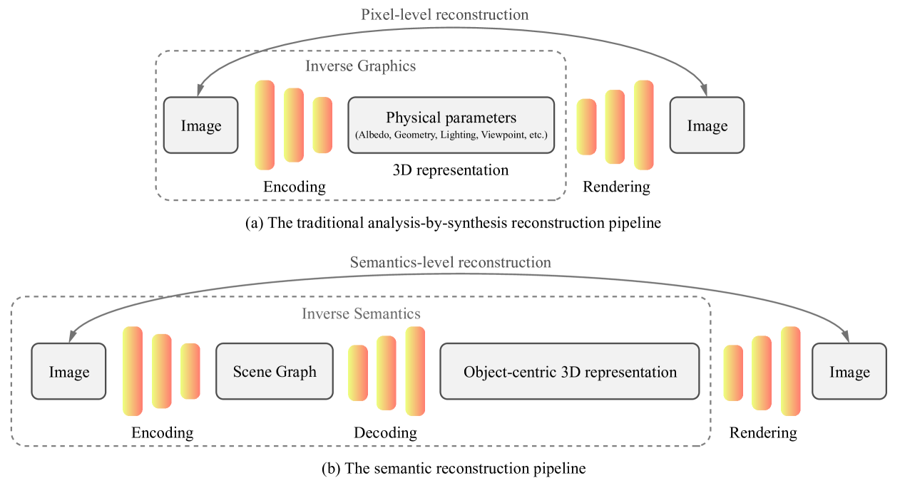
Figure 8: A paradigm comparison between inverse graphics and inverse semantics

Specifically, we can implement the inverse semantics paradigm with a GPT4V-guided GraphDreamer. We first use GPT4V to obtain the scene graph from an input image, and then apply GraphDreamer to generate a compositional 3D scene based on this scene graph. Enhanced by GPT4V’s powerful image understanding capabilities, we can obtain a detailed scene graph from the input image and generate a 3D scene from the graph that semantically inverses the given image. An qualitative example of our inverse semantics paradigm is provided in Figure9.

Figure 9: A qualitative example of the inverse semantics paradigm. We generate a scene graph directly from an input image with GPT4V and restrict the nodes present to the most salient ones. GPT4V identifies the objects and provides with proper attributes and edges for each object. This makes it possible to inverse modeling the semantics of a given scene image and extends the potential applications of GraphDreamer.

Moreover, it is also possible to extract rough estimates of the center coordinates of the objects in the graph from the image with GPT4V. The coordinate estimates are in 2D (the up-right plane) only, since the image is in 2D. For the third coordinate (on the front axis), GPT4V can offer the relative order by layering objects from the viewer’s perspective. Then, with the SDF representation of 3D objects, we can use these estimates as the sphere centers when initializing object SDFs u(i)⁢(𝐩)superscript 𝑢 𝑖 𝐩 u^{(i)}(\mathbf{p})italic_u start_POSTSUPERSCRIPT ( italic_i ) end_POSTSUPERSCRIPT ( bold_p ) to specify more accurately the spatial relationships of the objects, and thus to make the generated 3D scene better match the given image. We expect that the inverse semantics paradigm could be of general interest to the community, and our GPT4V-guided GraphDreamer serves as an important stepping stone towards this direction.

Figure 10: An example of more complex semantics represented with more nodes. ChatGPT structures the semantics in this complex image into a scene graph using the most salient node. To inverse such semantics and generated the scene in 3D, one may further ask GPT to provide with center coordinates for each node, which can make the semantic inverse more precise in terms of spatial relations.

Appendix D Failure Cases and Limitations

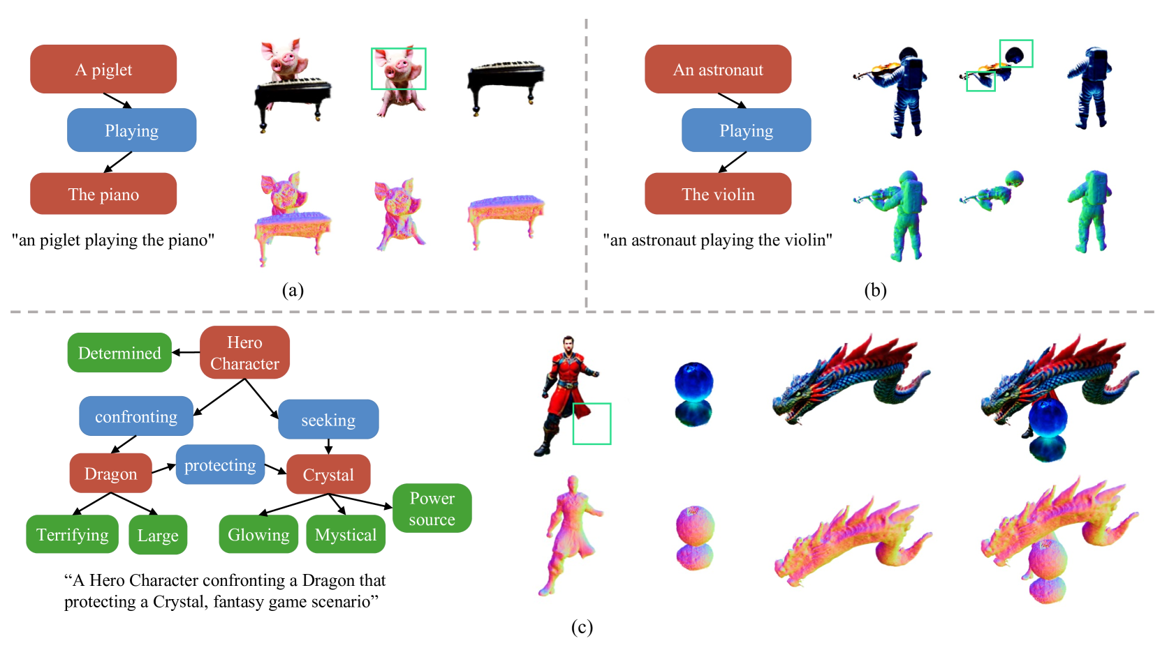
Figure 11: Examples of some failure cases. (a) In some cases, results of GraphDreamer may come with the Janus problem. (b) GraphDreamer failed to separate the violin from the astronaut’s left hand, which is closely held by that hand. (c) One leg of the Hero is missing. Part of these problems may stem from the SDS loss which only offers an approximate gradient (the Jacobian of Stable Diffusion is set to identity) and the known challenges when diffusion models deal with detailed parts. Optimizing multiple SDS losses Eq.(16) at the same time can also affect disentanglement. Enhanced supervision on object parts and improved prompts could help.

GraphDreamer still has some limitations. First, the generation quality of a single object is still largely limited by the SDS optimization. The commonly observed multi-head problems (i.e. missing, Janus problem) may also appear in GraphDreamer. See Figure11(a) for an example. The “piglet” in the generated results exhibits multiple heads from different viewpoints. Second, the decomposition of different objects may sometimes fail. See Figure11(b) for an example. We observe that the disentangled “astronaut” still looks like a reasonable astronaut, but the disentangled violin is affected by some parts of the astronaut. Third, the semantic meaning of some object in the scene may be incomplete. See Figure11(c) for an example. The hero character lacks a leg in the generated result.

We believe that part of these problems stem from the SDS loss which only offers an approximate gradient (the Jacobian of Stable Diffusion is set to identity) and the known challenges when diffusion models deal with detailed parts. We also suspect that optimizing multiple SDS losses Eq.(16) at the same time may affect disentanglement, and thus enhanced supervision on object parts and improved prompts could help.