2409/2409.00356.md

Title: Contrastive Augmentation: An Unsupervised Learning Approach for Keyword Spotting in Speech Technology

URL Source: https://arxiv.org/html/2409.00356

Markdown Content: 1 1 institutetext: Trine University, Phoenix, USA

1 1 email: wnd17460@gmail.com 2 2 institutetext: Boston University, Boston, USA

2 2 email: yjiang8@bu.edu 3 3 institutetext: Georgia Institute of Technology, Atlanta, GA, USA

3 3 email: yliu3689@gatech.edu 4 4 institutetext: Faculty of Computer Sciences, Dalhousie University, Halifax, Canada

4 4 email: jinkun.chen@dal.ca 5 5 institutetext: Texas A&M University, College Station, TX, USA

5 5 email: yolosun4488@gmail.com 6 6 institutetext: Georgia Institute of Technology, Atlanta, GA, USA

6 6 email: jinglei.tao@gatech.edu

Abstract

This paper addresses the persistent challenge in Keyword Spotting (KWS), a fundamental component in speech technology, regarding the acquisition of substantial labeled data for training. Given the difficulty in obtaining large quantities of positive samples and the laborious process of collecting new target samples when the keyword changes, we introduce a novel approach combining unsupervised contrastive learning and a unique augmentation-based technique. Our method allows the neural network to train on unlabeled data sets, potentially improving performance in downstream tasks with limited labeled data sets. We also propose that similar high-level feature representations should be employed for speech utterances with the same keyword despite variations in speed or volume. To achieve this, we present a speech augmentation-based unsupervised learning method that utilizes the similarity between the bottleneck layer feature and the audio reconstructing information for auxiliary training. Furthermore, we propose a compressed convolutional architecture to address potential redundancy and non-informative information in KWS tasks, enabling the model to simultaneously learn local features and focus on long-term information. This method achieves strong performance on the Google Speech Commands V2 Dataset. Inspired by recent advancements in sign spotting and spoken term detection, our method underlines the potential of our contrastive learning approach in KWS and the advantages of Query-by-Example Spoken Term Detection strategies. The presented CAB-KWS provide new perspectives in the field of KWS, demonstrating effective ways to reduce data collection efforts and increase the system’s robustness.

Keywords:

key word spotting contrastive learning unsupervised learning

1 INTRODUCTION

Keyword Spotting (KWS) is a fundamental application in the field of speech technology, playing a pivotal role in real-world scenarios, particularly in the context of interactive agents such as virtual assistants and voice-controlled devices. KWS is designed to detect a small set of pre-defined keywords within an audio stream. This capability is crucial for two primary reasons. First, it enables the initiation of interactions through specific commands like "hey Siri" or "OK, Google," effectively serving as an explicit cue for the system to start processing subsequent speech. Second, KWS can identify sensitive words within a conversation, thereby playing a vital role in protecting the privacy of the speaker. Given these applications, it is crucial to develop accurate and reliable KWS systems for effective real-world speech processing[9, 11, 18].

Despite the considerable advancements in KWS, a significant challenge that persists is the acquisition of sufficient labeled data for training. This is especially true for positive samples, which are often harder to obtain in large quantities. This issue is further exacerbated when the keyword changes, as it necessitates the collection of new target samples, a process that can be both time-consuming and resource-intensive. To address these challenges, we propose a novel approach that leverages the power of unsupervised contrastive learning and a unique augmentation-based method. Additionally, another potential problem is redundant information, speeches are noisy and complex, where only some key phrases are highly related to the keywords. However, convolutional methods treat all the word windows equally, ignoring that different words have different importance and should be weighted differently within word windows. Besides, the sliding windows used in the convolutional methods produce a lot of redundant information. Thus, it is important to reduce the non-informative and redundant information and distinguish the contributions of different convolutional features.

Our method enables the neural network to be trained on unlabeled datasets, reducing the reliance on extensive labeled data. This technique can greatly enhance the performance of downstream tasks, even in scenarios where labeled datasets are scarce. Additionally, we propose that speech utterances containing the same keyword, regardless of variations in speed or volume, should exhibit similar high-level feature representations in KWS tasks. To achieve this, we present a speech augmentation-based unsupervised learning approach. This method leverages the similarity of bottleneck layer features, along with audio reconstruction information, for auxiliary training to improve system robustness.

In addition to these innovations, we propose a compressed convolutional architecture for the KWS task. This architecture, designed to tackle the issue of redundant information, has demonstrated strong performance on the Google Speech Commands V2 Dataset. By doing so, it enables the model to learn local features and focus on long-term information simultaneously, thereby enhancing its performance on the KWS task.

Our approach is inspired by recent advancements in the field of sign spotting and spoken term detection. For instance, Varol et al.[21] demonstrated the effectiveness of Noise Contrastive Estimation and Multiple Instance Learning in sign spotting, which could provide insights into the use of contrastive learning in KWS. Similarly, the works of Tejedor et al.[19, 20] on Query-by-Example Spoken Term Detection (QbE STD) highlight the potential of QbE STD strategies in outperforming text-based STD in unseen data domains, reinforcing the potential advantages of our proposed method.

Our major contributions in this work are as follows:

• • We introduce a compact convolutional architecture for the KWS task that achieves strong results on the Google Speech Commands V2 Dataset.

• • We develop an unsupervised loss and a contrastive loss to evaluate the similarity between original and augmented speech, as well as the proximity within each minibatch.

• • We introduce a speech augmentation-based unsupervised learning approach, utilizing the similarity between the bottleneck layer feature, as well as the audio reconstructing information for auxiliary training.

Theremainder of this paper is structured as follows. Section2 provides an overview of related work in the areas of data augmentation, unsupervised learning, and other methodologies of KWS tasks. Section3 offers a background on contrastive learning. Section4 details the proposed model architecture and our augmentation-based unsupervised contrastive learning loss. Section5 discusses the configuration, research questions, and experimental setups. Section6 presents the experimental results and compares them with other pre-training methods. We also discuss the relationship between pre-training steps and the performance of downstream KWS tasks. Finally, Section7 concludes the paper with a summary of our findings and potential avenues for future work.

2 RELATED WORK

Data augmentation is widely acknowledged as an effective technique for enriching the training datasets in speech applications, such as Automatic Speech Recognition (ASR) and Keyword Spotting (KWS). Various methods have been explored, such as vocal tract length perturbation[5], speed-perturbation[8], and the introduction of noisy audio signals[4]. More recently, spectral-domain augmentation techniques, such as SpecAugment[15] and WavAugment[7], have been developed to further improve the robustness of speech recognition systems. In this work, we extend these efforts by applying speed and volume perturbation in our speech augmentation method.

While supervised learning has been the primary approach in the KWS area, it often requires large amounts of labeled data, which can be challenging to obtain, especially for less frequently used languages. This has sparked growing interest in weakly supervised and unsupervised approaches. For example, Noisy Student Training, a semi-supervised learning technique, has been employed in ASR[16] and subsequently adapted for robust keyword spotting[17]. Additionally, unsupervised methods for KWS have been investigated[3, 10, 25], yielding promising outcomes. Building on these efforts, we propose an unsupervised learning framework for the keyword spotting task in this paper.

The Google Speech Commands V2 Dataset is a widely used benchmark for novel ideas in KWS. Numerous works have performed experiments on this dataset, introducing various architectures and methods. For instance, a convolutional recurrent network with attention was introduced by [2], and a deep residual network, MatchboxNet, was proposed by [12]. More recently, an edge computing-focused model called EdgeCRNN[24] was introduced, along with a method that integrates triplet loss-based embeddings with a modified K-Nearest Neighbor (KNN) for classification[22]. In this work, we also evaluate our speech augmentation-based unsupervised learning method on this dataset and compare it with other unsupervised approaches, including CPC[13], APC[1], and MPC [6].

3 PRELIMINARY STUDY OF CONTRASTIVE LEARNING

In the context of a classification task involving K 𝐾 K italic_K classes, we consider a dataset {𝒙 i,y i}i=1 N superscript subscript subscript 𝒙 𝑖 subscript 𝑦 𝑖 𝑖 1 𝑁\left{\boldsymbol{x}{i},y{i}\right}{i=1}^{N}{ bold_italic_x start_POSTSUBSCRIPT italic_i end_POSTSUBSCRIPT , italic_y start_POSTSUBSCRIPT italic_i end_POSTSUBSCRIPT } start_POSTSUBSCRIPT italic_i = 1 end_POSTSUBSCRIPT start_POSTSUPERSCRIPT italic_N end_POSTSUPERSCRIPT with N 𝑁 N italic_N training samples. Each 𝒙⁢i∈ℝ L 𝒙 𝑖 superscript ℝ 𝐿\boldsymbol{x}{i}\in\mathbb{R}^{L}bold_italic_x italic_i ∈ blackboard_R start_POSTSUPERSCRIPT italic_L end_POSTSUPERSCRIPT represents an input sentence of L 𝐿 L italic_L words, and each y i∈1,2,⋯,K subscript 𝑦 𝑖 1 2⋯𝐾 y{i}\in{1,2,\cdots,K}italic_y start_POSTSUBSCRIPT italic_i end_POSTSUBSCRIPT ∈ 1 , 2 , ⋯ , italic_K is the corresponding label. We denote the set of training sample indexes by ℐ=1,2,⋯,N ℐ 1 2⋯𝑁\mathcal{I}={1,2,\cdots,N}caligraphic_I = 1 , 2 , ⋯ , italic_N and the set of label indexes by 𝒦=1,2,⋯,K 𝒦 1 2⋯𝐾\mathcal{K}={1,2,\cdots,K}caligraphic_K = 1 , 2 , ⋯ , italic_K.

We explore the realm of self-supervised contrastive learning, a technique that has demonstrated its effectiveness in numerous studies. Given N 𝑁 N italic_N training samples {𝒙 i}i=1 N superscript subscript subscript 𝒙 𝑖 𝑖 1 𝑁\left{\boldsymbol{x}{i}\right}{i=1}^{N}{ bold_italic_x start_POSTSUBSCRIPT italic_i end_POSTSUBSCRIPT } start_POSTSUBSCRIPT italic_i = 1 end_POSTSUBSCRIPT start_POSTSUPERSCRIPT italic_N end_POSTSUPERSCRIPT with a number of augmented samples, the standard contrastive loss is defined as follows:

ℒ⁢self=1 N⁢∑i∈ℐ−log⁡exp⁡(𝒛⁢i⋅𝒛⁢j⁢(i)/τ)∑a∈𝒜⁢i exp⁡(𝒛⁢i⋅𝒛 a/τ)ℒ self 1 𝑁 𝑖 ℐ⋅𝒛 𝑖 𝒛 𝑗 𝑖 𝜏 subscript 𝑎 𝒜 𝑖⋅𝒛 𝑖 subscript 𝒛 𝑎 𝜏\mathcal{L}{\text{self }}=\frac{1}{N}\sum{i\in\mathcal{I}}-\log\frac{\exp\left% (\boldsymbol{z}{i}\cdot\boldsymbol{z}{j(i)}/\tau\right)}{\sum_{a\in\mathcal{A}% {i}}\exp\left(\boldsymbol{z}{i}\cdot\boldsymbol{z}_{a}/\tau\right)}caligraphic_L self = divide start_ARG 1 end_ARG start_ARG italic_N end_ARG ∑ italic_i ∈ caligraphic_I - roman_log divide start_ARG roman_exp ( bold_italic_z italic_i ⋅ bold_italic_z italic_j ( italic_i ) / italic_τ ) end_ARG start_ARG ∑ start_POSTSUBSCRIPT italic_a ∈ caligraphic_A italic_i end_POSTSUBSCRIPT roman_exp ( bold_italic_z italic_i ⋅ bold_italic_z start_POSTSUBSCRIPT italic_a end_POSTSUBSCRIPT / italic_τ ) end_ARG(1)

Here, 𝒛⁢i 𝒛 𝑖\boldsymbol{z}{i}bold_italic_z italic_i is the normalized representation of 𝒙⁢i,𝒜 i:=ℐ\i assign 𝒙 𝑖 subscript 𝒜 𝑖\ℐ 𝑖\boldsymbol{x}{i},\mathcal{A}_{i}:=\mathcal{I}\backslash{i}bold_italic_x italic_i , caligraphic_A start_POSTSUBSCRIPT italic_i end_POSTSUBSCRIPT := caligraphic_I \ italic_i is the set of indexes of the contrastive samples, the ⋅⋅\cdot⋅ symbol denotes the dot product, and τ∈ℝ+𝜏 superscript ℝ\tau\in\mathbb{R}^{+}italic_τ ∈ blackboard_R start_POSTSUPERSCRIPT + end_POSTSUPERSCRIPT is the temperature factor.

However, self-supervised contrastive learning does not utilize supervised signals. A previous study [Khosla et al., 2020] incorporated supervision into contrastive learning in a straightforward manner. It simply treated samples from the same class as positive samples and samples from different classes as negative samples. The following contrastive loss is defined for supervised tasks:

ℒ⁢sup=1 N⁢∑i∈ℐ⁢1|𝒫⁢i|⁢∑p∈𝒫⁢i−log⁡exp⁡(𝒛⁢i⋅𝒛⁢p/τ)∑a∈𝒜⁢i⁢exp⁡(𝒛⁢i⋅𝒛 a/τ)ℒ sup 1 𝑁 𝑖 ℐ 1 𝒫 𝑖 𝑝 𝒫 𝑖⋅𝒛 𝑖 𝒛 𝑝 𝜏 𝑎 𝒜 𝑖⋅𝒛 𝑖 subscript 𝒛 𝑎 𝜏\mathcal{L}{\text{sup }}=\frac{1}{N}\sum{i\in\mathcal{I}}\frac{1}{\left|% \mathcal{P}{i}\right|}\sum{p\in\mathcal{P}{i}}-\log\frac{\exp\left(\boldsymbol% {z}{i}\cdot\boldsymbol{z}{p}/\tau\right)}{\sum{a\in\mathcal{A}{i}}\exp\left(% \boldsymbol{z}{i}\cdot\boldsymbol{z}_{a}/\tau\right)}caligraphic_L sup = divide start_ARG 1 end_ARG start_ARG italic_N end_ARG ∑ italic_i ∈ caligraphic_I divide start_ARG 1 end_ARG start_ARG | caligraphic_P italic_i | end_ARG ∑ italic_p ∈ caligraphic_P italic_i - roman_log divide start_ARG roman_exp ( bold_italic_z italic_i ⋅ bold_italic_z italic_p / italic_τ ) end_ARG start_ARG ∑ italic_a ∈ caligraphic_A italic_i roman_exp ( bold_italic_z italic_i ⋅ bold_italic_z start_POSTSUBSCRIPT italic_a end_POSTSUBSCRIPT / italic_τ ) end_ARG(2)

Despite its effectiveness, this approach still requires learning a linear classifier using the cross-entropy loss apart from the contrastive term. This is because the contrastive loss can only learn generic representations for the input examples. Thus, we argue that the supervised contrastive learning developed so far appears to be a naive adaptation of unsupervised contrastive learning to the classification

4 Proposed Method

The keyword spotting task can be framed as a sequence classification problem, where the keyword spotting network maps an input audio sequence X={x 0,x 1,…,x T}𝑋 subscript 𝑥 0 subscript 𝑥 1…subscript 𝑥 𝑇 X=\left{x_{0},x_{1},\ldots,x_{T}\right}italic_X = { italic_x start_POSTSUBSCRIPT 0 end_POSTSUBSCRIPT , italic_x start_POSTSUBSCRIPT 1 end_POSTSUBSCRIPT , … , italic_x start_POSTSUBSCRIPT italic_T end_POSTSUBSCRIPT } to a set of keyword classes Y∈y 1:S 𝑌 subscript 𝑦:1 𝑆 Y\in y_{1:S}italic_Y ∈ italic_y start_POSTSUBSCRIPT 1 : italic_S end_POSTSUBSCRIPT. Here, T 𝑇 T italic_T represents the number of frames, and S 𝑆 S italic_S denotes the number of classes. Our proposed keyword spotting model, depicted in Fig LABEL:fig(A), consists of five key components: (1) Compressed Convolutional Layer, (2) Transformer Block, (3) Feature Selection Layer, (4) Bottleneck Layer, and (5) Projection Layer.

4.1 Compressed Convolutional Layer

The Compressed Convolutional Layer replaces the CNN block in the original design. This layer learns dense and informative frame representations from the input sequence X 𝑋 X italic_X. Specifically, it utilizes convolutional neural networks (CNNs), an attention-based soft-pooling approach, and residual convolution blocks for feature extraction and compression.

4.1.1 Frame Convolution

Just as in the original CNN block, the convolution operation is applied to each frame. Given the input sequence X 𝑋 X italic_X and the i 𝑖 i italic_i-th filter, the convolution for the j 𝑗 j italic_j-th frame is expressed as

𝐱 j i=conv⁡({𝐱 j,𝐱 j+1,⋯,𝐱 j+k i−1};𝐖 x i),superscript subscript 𝐱 𝑗 𝑖 conv subscript 𝐱 𝑗 subscript 𝐱 𝑗 1⋯subscript 𝐱 𝑗 subscript 𝑘 𝑖 1 superscript subscript 𝐖 𝑥 𝑖\mathbf{x}{j}^{i}=\operatorname{conv}\left(\left{\mathbf{x}{j},\mathbf{x}{% j+1},\cdots,\mathbf{x}{j+k_{i}-1}\right};\mathbf{W}_{x}^{i}\right),bold_x start_POSTSUBSCRIPT italic_j end_POSTSUBSCRIPT start_POSTSUPERSCRIPT italic_i end_POSTSUPERSCRIPT = roman_conv ( { bold_x start_POSTSUBSCRIPT italic_j end_POSTSUBSCRIPT , bold_x start_POSTSUBSCRIPT italic_j + 1 end_POSTSUBSCRIPT , ⋯ , bold_x start_POSTSUBSCRIPT italic_j + italic_k start_POSTSUBSCRIPT italic_i end_POSTSUBSCRIPT - 1 end_POSTSUBSCRIPT } ; bold_W start_POSTSUBSCRIPT italic_x end_POSTSUBSCRIPT start_POSTSUPERSCRIPT italic_i end_POSTSUPERSCRIPT ) ,(3)

where 𝐖 x i superscript subscript 𝐖 𝑥 𝑖\mathbf{W}_{x}^{i}bold_W start_POSTSUBSCRIPT italic_x end_POSTSUBSCRIPT start_POSTSUPERSCRIPT italic_i end_POSTSUPERSCRIPT is the learned parameter of the i 𝑖 i italic_i-th filter.

4.1.2 Attention-based Soft-pooling

To eliminate redundant information in the speech dataset, we propose an attention-based soft-pooling operation on the frame representations learned by the previous equation. Specifically, given a frame x j subscript 𝑥 𝑗 x_{j}italic_x start_POSTSUBSCRIPT italic_j end_POSTSUBSCRIPT, its neighboring frames {x j+1,⋯,x j+g−1}subscript 𝑥 𝑗 1⋯subscript 𝑥 𝑗 𝑔 1\left{x_{j+1},\cdots,x_{j+g-1}\right}{ italic_x start_POSTSUBSCRIPT italic_j + 1 end_POSTSUBSCRIPT , ⋯ , italic_x start_POSTSUBSCRIPT italic_j + italic_g - 1 end_POSTSUBSCRIPT }, and the corresponding filter f i subscript 𝑓 𝑖 f_{i}italic_f start_POSTSUBSCRIPT italic_i end_POSTSUBSCRIPT, we first learn the local-based attention scores α j i=𝐖 α i⁢𝐱 j i+b superscript subscript 𝛼 𝑗 𝑖 superscript subscript 𝐖 𝛼 𝑖 superscript subscript 𝐱 𝑗 𝑖 𝑏\alpha_{j}^{i}=\mathbf{W}{\alpha}^{i}\mathbf{x}{j}^{i}+b italic_α start_POSTSUBSCRIPT italic_j end_POSTSUBSCRIPT start_POSTSUPERSCRIPT italic_i end_POSTSUPERSCRIPT = bold_W start_POSTSUBSCRIPT italic_α end_POSTSUBSCRIPT start_POSTSUPERSCRIPT italic_i end_POSTSUPERSCRIPT bold_x start_POSTSUBSCRIPT italic_j end_POSTSUBSCRIPT start_POSTSUPERSCRIPT italic_i end_POSTSUPERSCRIPT + italic_b with softmax function, and then conduct the soft-pooling operation to obtain the compressed representation as in the following equation:

𝐨 p i=∑q=j j+g−1 β q i⁢𝐱 q i superscript subscript 𝐨 𝑝 𝑖 superscript subscript 𝑞 𝑗 𝑗 𝑔 1 superscript subscript 𝛽 𝑞 𝑖 superscript subscript 𝐱 𝑞 𝑖\mathbf{o}{p}^{i}=\sum{q=j}^{j+g-1}\beta_{q}^{i}\mathbf{x}_{q}^{i}bold_o start_POSTSUBSCRIPT italic_p end_POSTSUBSCRIPT start_POSTSUPERSCRIPT italic_i end_POSTSUPERSCRIPT = ∑ start_POSTSUBSCRIPT italic_q = italic_j end_POSTSUBSCRIPT start_POSTSUPERSCRIPT italic_j + italic_g - 1 end_POSTSUPERSCRIPT italic_β start_POSTSUBSCRIPT italic_q end_POSTSUBSCRIPT start_POSTSUPERSCRIPT italic_i end_POSTSUPERSCRIPT bold_x start_POSTSUBSCRIPT italic_q end_POSTSUBSCRIPT start_POSTSUPERSCRIPT italic_i end_POSTSUPERSCRIPT(4)

4.1.3 Residual Convolution Block

We now have a denoised matrix {𝐨 1 i,𝐨 2 i,⋯,𝐨 P i}superscript subscript 𝐨 1 𝑖 superscript subscript 𝐨 2 𝑖⋯superscript subscript 𝐨 𝑃 𝑖\left{\mathbf{o}{1}^{i},\mathbf{o}{2}^{i},\cdots,\mathbf{o}_{P}^{i}\right}{ bold_o start_POSTSUBSCRIPT 1 end_POSTSUBSCRIPT start_POSTSUPERSCRIPT italic_i end_POSTSUPERSCRIPT , bold_o start_POSTSUBSCRIPT 2 end_POSTSUBSCRIPT start_POSTSUPERSCRIPT italic_i end_POSTSUPERSCRIPT , ⋯ , bold_o start_POSTSUBSCRIPT italic_P end_POSTSUBSCRIPT start_POSTSUPERSCRIPT italic_i end_POSTSUPERSCRIPT } that represents the input sequence X 𝑋 X italic_X. To avoid vanishing gradients and facilitate model training, we introduce residual blocks on top of the compressed features. In particular, we replace the batch norm layer with the group norm layer. Let a 𝑎 a italic_a denotes the number of residual blocks, we have

𝐫 p i=ResidualBlcok⁡({𝐨 p i,⋯,𝐨 p+a−1 i}),superscript subscript 𝐫 𝑝 𝑖 ResidualBlcok superscript subscript 𝐨 𝑝 𝑖⋯superscript subscript 𝐨 𝑝 𝑎 1 𝑖\mathbf{r}{p}^{i}=\operatorname{ResidualBlcok}\left(\left{\mathbf{o}{p}^{i}% ,\cdots,\mathbf{o}_{p+a-1}^{i}\right}\right),bold_r start_POSTSUBSCRIPT italic_p end_POSTSUBSCRIPT start_POSTSUPERSCRIPT italic_i end_POSTSUPERSCRIPT = roman_ResidualBlcok ( { bold_o start_POSTSUBSCRIPT italic_p end_POSTSUBSCRIPT start_POSTSUPERSCRIPT italic_i end_POSTSUPERSCRIPT , ⋯ , bold_o start_POSTSUBSCRIPT italic_p + italic_a - 1 end_POSTSUBSCRIPT start_POSTSUPERSCRIPT italic_i end_POSTSUPERSCRIPT } ) ,(5)

where ResidualBlock ResidualBlock\operatorname{ResidualBlock}roman_ResidualBlock is the operation of the residual convolution block.

4.2 ResLayer Block

4.2.1 Transformer Block

The output from the Compressed Convolutional Layer, R={𝐫 1 i,𝐫 2 i,⋯,𝐫 P i}𝑅 superscript subscript 𝐫 1 𝑖 superscript subscript 𝐫 2 𝑖⋯superscript subscript 𝐫 𝑃 𝑖 R=\left{\mathbf{r}{1}^{i},\mathbf{r}{2}^{i},\cdots,\mathbf{r}{P}^{i}\right}italic_R = { bold_r start_POSTSUBSCRIPT 1 end_POSTSUBSCRIPT start_POSTSUPERSCRIPT italic_i end_POSTSUPERSCRIPT , bold_r start_POSTSUBSCRIPT 2 end_POSTSUBSCRIPT start_POSTSUPERSCRIPT italic_i end_POSTSUPERSCRIPT , ⋯ , bold_r start_POSTSUBSCRIPT italic_P end_POSTSUBSCRIPT start_POSTSUPERSCRIPT italic_i end_POSTSUPERSCRIPT }, is then fed into the Transformer Block. This block captures long-term dependencies in the sequence via the self-attention mechanism: E t⁢r⁢a⁢n=Self-Attention×M⁢(R),subscript 𝐸 𝑡 𝑟 𝑎 𝑛 subscript Self-Attention absent 𝑀 𝑅 E{tran}=\text{ Self-Attention }_{\times M}\left(R\right),italic_E start_POSTSUBSCRIPT italic_t italic_r italic_a italic_n end_POSTSUBSCRIPT = Self-Attention start_POSTSUBSCRIPT × italic_M end_POSTSUBSCRIPT ( italic_R ) , where M 𝑀 M italic_M is the number of self-attention layers.

4.2.2 Feature Selecting Layer

Following the Transformer Block, the Feature Selecting Layer is implemented to extract keyword information from the sequence E t⁢r⁢a⁢n subscript 𝐸 𝑡 𝑟 𝑎 𝑛 E_{tran}italic_E start_POSTSUBSCRIPT italic_t italic_r italic_a italic_n end_POSTSUBSCRIPT.

E feat=Concat⁡(E tran⁢[T−r,T]),subscript 𝐸 feat Concat subscript 𝐸 tran 𝑇 𝑟 𝑇 E_{\text{feat }}=\operatorname{Concat}\left(E_{\text{tran }}[T-r,T]\right),italic_E start_POSTSUBSCRIPT feat end_POSTSUBSCRIPT = roman_Concat ( italic_E start_POSTSUBSCRIPT tran end_POSTSUBSCRIPT [ italic_T - italic_r , italic_T ] ) ,(6)

Here, the last r 𝑟 r italic_r frames of E t⁢r⁢a⁢n subscript 𝐸 𝑡 𝑟 𝑎 𝑛 E_{tran}italic_E start_POSTSUBSCRIPT italic_t italic_r italic_a italic_n end_POSTSUBSCRIPT are gathered, and all the collected frames are concatenated together into one feature vector E f⁢e⁢a⁢t subscript 𝐸 𝑓 𝑒 𝑎 𝑡 E_{feat}italic_E start_POSTSUBSCRIPT italic_f italic_e italic_a italic_t end_POSTSUBSCRIPT.

4.2.3 Bottleneck and Project Layers

After the Feature Selecting Layer, a Bottleneck Layer and a Projection Layer are added. These layers map the hidden states to the predicted classification classes Y~~𝑌\tilde{Y}over~ start_ARG italic_Y end_ARG.

E b⁢n=FC bn⁢(E feat),subscript 𝐸 𝑏 𝑛 subscript FC bn subscript 𝐸 feat E_{bn}=\mathrm{FC}{\mathrm{bn}}\left(E{\text{feat }}\right),italic_E start_POSTSUBSCRIPT italic_b italic_n end_POSTSUBSCRIPT = roman_FC start_POSTSUBSCRIPT roman_bn end_POSTSUBSCRIPT ( italic_E start_POSTSUBSCRIPT feat end_POSTSUBSCRIPT ) ,(7)

Y=FC proj⁢(E b⁢n),𝑌 subscript FC proj subscript 𝐸 𝑏 𝑛\tilde{Y}=\mathrm{FC}{\operatorname{proj}}\left(E{bn}\right),over~ start_ARG italic_Y end_ARG = roman_FC start_POSTSUBSCRIPT roman_proj end_POSTSUBSCRIPT ( italic_E start_POSTSUBSCRIPT italic_b italic_n end_POSTSUBSCRIPT ) ,(8)

Finally, the cross-entropy (CE) loss for supervised learning and model fine-tuning is computed based on the predicted classes Y~~𝑌\tilde{Y}over~ start_ARG italic_Y end_ARG and ground truth classes Y 𝑌 Y italic_Y. ℒ c⁢e=CE⁡(Y,Y)subscript ℒ 𝑐 𝑒 CE 𝑌𝑌\mathcal{L}_{ce}=\operatorname{CE}(Y,\tilde{Y})caligraphic_L start_POSTSUBSCRIPT italic_c italic_e end_POSTSUBSCRIPT = roman_CE ( italic_Y , over~ start_ARG italic_Y end_ARG ).

Figure 1: A: The architecture of our CAB-KWS for the keyword spotting task consists of a compressed layer, ResLayer Block, and Decision Block. B: The proposed method integrates speech augmentation with unsupervised and contrastive learning for audio processing.

4.3 Augmentation Method

Data augmentation is a widely utilized technique to enhance model performance and robustness, particularly in speech-related tasks. In this study, we delve into speed and volume-based augmentation in the context of unsupervised learning for keyword detection. A specific audio sequence, represented as X=A⁢(t)𝑋 𝐴 𝑡 X=A(t)italic_X = italic_A ( italic_t ), is defined by its amplitude A 𝐴 A italic_A and time index t 𝑡 t italic_t.

Regarding speed augmentation, a speed ratio symbolized by λ speed subscript 𝜆 speed\lambda_{\text{speed }}italic_λ start_POSTSUBSCRIPT speed end_POSTSUBSCRIPT is established to modify the speed of X 𝑋 X italic_X. The following formula describes this process:X a⁢u⁢g=A⁢(λ speed⁢t)superscript 𝑋 𝑎 𝑢 𝑔 𝐴 subscript 𝜆 speed 𝑡 X^{aug}=A\left(\lambda_{\text{speed }}t\right)italic_X start_POSTSUPERSCRIPT italic_a italic_u italic_g end_POSTSUPERSCRIPT = italic_A ( italic_λ start_POSTSUBSCRIPT speed end_POSTSUBSCRIPT italic_t ). For volume augmentation, similarly, we set an intensity ratio, λ volume subscript 𝜆 volume\lambda_{\text{volume }}italic_λ start_POSTSUBSCRIPT volume end_POSTSUBSCRIPT, to alter the volume of X 𝑋 X italic_X, as presented in the following equation: X a⁢u⁢g=λ volume⁢A⁢(t)superscript 𝑋 𝑎 𝑢 𝑔 subscript 𝜆 volume 𝐴 𝑡 X^{aug}=\lambda_{\text{volume }}A(t)italic_X start_POSTSUPERSCRIPT italic_a italic_u italic_g end_POSTSUPERSCRIPT = italic_λ start_POSTSUBSCRIPT volume end_POSTSUBSCRIPT italic_A ( italic_t ). By using various ratios λ speed subscript 𝜆 speed\lambda_{\text{speed }}italic_λ start_POSTSUBSCRIPT speed end_POSTSUBSCRIPT and λ volume subscript 𝜆 volume\lambda_{\text{volume }}italic_λ start_POSTSUBSCRIPT volume end_POSTSUBSCRIPT, we can generate multiple pairs of speech sequences, (X,X a⁢u⁢g)𝑋 superscript 𝑋 𝑎 𝑢 𝑔\left(X,X^{aug}\right)( italic_X , italic_X start_POSTSUPERSCRIPT italic_a italic_u italic_g end_POSTSUPERSCRIPT ), to facilitate the training of the audio representation network via unsupervised learning. The fundamental assumption is that speech utterances, regardless of speed or volume variations, should exhibit similar high-level feature representations for keyword-spotting tasks.

4.4 Contrastive Learning Loss

We aim to align the softmax transform of the dot product between the feature representation 𝒛⁢i 𝒛 𝑖\boldsymbol{z}{i}bold_italic_z italic_i and the classifier 𝜽⁢i 𝜽 𝑖\boldsymbol{\theta}{i}bold_italic_θ italic_i of the input example X i subscript 𝑋 𝑖 X_{i}italic_X start_POSTSUBSCRIPT italic_i end_POSTSUBSCRIPT with its corresponding label. Let 𝜽⁢i∗𝜽 superscript 𝑖\boldsymbol{\theta}{i}^{*}bold_italic_θ italic_i start_POSTSUPERSCRIPT ∗ end_POSTSUPERSCRIPT denote the column of 𝜽⁢i 𝜽 𝑖\boldsymbol{\theta}{i}bold_italic_θ italic_i that corresponds to the ground-truth label of 𝒙⁢i 𝒙 𝑖\boldsymbol{x}{i}bold_italic_x italic_i. We aim to maximize the dot product 𝜽⁢i∗T⁢𝒛⁢i 𝜽 superscript 𝑖 absent 𝑇 𝒛 𝑖\boldsymbol{\theta}{i}^{*T}\boldsymbol{z}{i}bold_italic_θ italic_i start_POSTSUPERSCRIPT ∗ italic_T end_POSTSUPERSCRIPT bold_italic_z italic_i. To achieve this, we learn a better representation of 𝜽⁢i 𝜽 𝑖\boldsymbol{\theta}{i}bold_italic_θ italic_i and 𝒛 i subscript 𝒛 𝑖\boldsymbol{z}_{i}bold_italic_z start_POSTSUBSCRIPT italic_i end_POSTSUBSCRIPT using supervised signals.

The Dual Contrastive Loss exploits the relation between different training samples to maximize 𝜽⁢i∗T⁢𝒛⁢j 𝜽 superscript 𝑖 absent 𝑇 𝒛 𝑗\boldsymbol{\theta}{i}^{*T}\boldsymbol{z}{j}bold_italic_θ italic_i start_POSTSUPERSCRIPT ∗ italic_T end_POSTSUPERSCRIPT bold_italic_z italic_j if 𝒙⁢j 𝒙 𝑗\boldsymbol{x}{j}bold_italic_x italic_j has the same label as 𝒙⁢i 𝒙 𝑖\boldsymbol{x}{i}bold_italic_x italic_i, while minimizing 𝜽⁢i∗T⁢𝒛⁢j 𝜽 superscript 𝑖 absent 𝑇 𝒛 𝑗\boldsymbol{\theta}{i}^{*T}\boldsymbol{z}{j}bold_italic_θ italic_i start_POSTSUPERSCRIPT ∗ italic_T end_POSTSUPERSCRIPT bold_italic_z italic_j if 𝒙⁢j 𝒙 𝑗\boldsymbol{x}{j}bold_italic_x italic_j carries a different label from 𝒙⁢i 𝒙 𝑖\boldsymbol{x}{i}bold_italic_x italic_i.

To define the contrastive loss, given an anchor 𝒛⁢i 𝒛 𝑖\boldsymbol{z}{i}bold_italic_z italic_i originating from the input example 𝒙⁢i 𝒙 𝑖\boldsymbol{x}{i}bold_italic_x italic_i, we take {𝜽 j∗}j∈𝒫 i subscript superscript subscript 𝜽 𝑗 𝑗 subscript 𝒫 𝑖\left{\boldsymbol{\theta}{j}^{*}\right}{j\in\mathcal{P}{i}}{ bold_italic_θ start_POSTSUBSCRIPT italic_j end_POSTSUBSCRIPT start_POSTSUPERSCRIPT ∗ end_POSTSUPERSCRIPT } start_POSTSUBSCRIPT italic_j ∈ caligraphic_P start_POSTSUBSCRIPT italic_i end_POSTSUBSCRIPT end_POSTSUBSCRIPT as positive samples and {𝜽 j∗}j∈𝒜 i\𝒫 i subscript superscript subscript 𝜽 𝑗 𝑗\subscript 𝒜 𝑖 subscript 𝒫 𝑖\left{\boldsymbol{\theta}{j}^{*}\right}{j\in\mathcal{A}{i}\backslash% \mathcal{P}_{i}}{ bold_italic_θ start_POSTSUBSCRIPT italic_j end_POSTSUBSCRIPT start_POSTSUPERSCRIPT ∗ end_POSTSUPERSCRIPT } start_POSTSUBSCRIPT italic_j ∈ caligraphic_A start_POSTSUBSCRIPT italic_i end_POSTSUBSCRIPT \ caligraphic_P start_POSTSUBSCRIPT italic_i end_POSTSUBSCRIPT end_POSTSUBSCRIPT as negative samples. The contrastive loss is defined as follows:

ℒ⁢z=1 N⁢∑i∈ℐ⁢1|𝒫⁢i|⁢∑p∈𝒫⁢i−log⁡exp⁡(𝜽⁢p⋅𝒛⁢i/τ)∑a∈𝒜⁢i⁢exp⁡(𝜽⁢a⋅𝒛 i/τ)ℒ 𝑧 1 𝑁 𝑖 ℐ 1 𝒫 𝑖 𝑝 𝒫 𝑖⋅𝜽 𝑝 𝒛 𝑖 𝜏 𝑎 𝒜 𝑖⋅𝜽 𝑎 subscript 𝒛 𝑖 𝜏\mathcal{L}{z}=\frac{1}{N}\sum{i\in\mathcal{I}}\frac{1}{\left|\mathcal{P}{i}% \right|}\sum{p\in\mathcal{P}{i}}-\log\frac{\exp\left(\boldsymbol{\theta}{p}% \cdot\boldsymbol{z}{i}/\tau\right)}{\sum{a\in\mathcal{A}{i}}\exp\left(% \boldsymbol{\theta}{a}\cdot\boldsymbol{z}_{i}/\tau\right)}caligraphic_L italic_z = divide start_ARG 1 end_ARG start_ARG italic_N end_ARG ∑ italic_i ∈ caligraphic_I divide start_ARG 1 end_ARG start_ARG | caligraphic_P italic_i | end_ARG ∑ italic_p ∈ caligraphic_P italic_i - roman_log divide start_ARG roman_exp ( bold_italic_θ italic_p ⋅ bold_italic_z italic_i / italic_τ ) end_ARG start_ARG ∑ italic_a ∈ caligraphic_A italic_i roman_exp ( bold_italic_θ italic_a ⋅ bold_italic_z start_POSTSUBSCRIPT italic_i end_POSTSUBSCRIPT / italic_τ ) end_ARG(9)

Here, τ∈ℝ+𝜏 superscript ℝ\tau\in\mathbb{R}^{+}italic_τ ∈ blackboard_R start_POSTSUPERSCRIPT + end_POSTSUPERSCRIPT is the temperature factor, 𝒜⁢i:=ℐ\i assign 𝒜 𝑖\ℐ 𝑖\mathcal{A}{i}:=\mathcal{I}\backslash{i}caligraphic_A italic_i := caligraphic_I \ italic_i is the set of indexes of the contrastive samples, 𝒫 i:={p∈𝒜 i:y p=y i}assign subscript 𝒫 𝑖 conditional-set 𝑝 subscript 𝒜 𝑖 subscript 𝑦 𝑝 subscript 𝑦 𝑖\mathcal{P}{i}:=\left{p\in\mathcal{A}{i}:y_{p}=y_{i}\right}caligraphic_P start_POSTSUBSCRIPT italic_i end_POSTSUBSCRIPT := { italic_p ∈ caligraphic_A start_POSTSUBSCRIPT italic_i end_POSTSUBSCRIPT : italic_y start_POSTSUBSCRIPT italic_p end_POSTSUBSCRIPT = italic_y start_POSTSUBSCRIPT italic_i end_POSTSUBSCRIPT } is the set of indexes of positive samples, and |𝒫⁢i|𝒫 𝑖\left|\mathcal{P}{i}\right|| caligraphic_P italic_i | is the cardinality of 𝒫⁢i 𝒫 𝑖\mathcal{P}{i}caligraphic_P italic_i. Similarly, given an anchor 𝜽⁢i∗𝜽 superscript 𝑖\boldsymbol{\theta}{i}^{*}bold_italic_θ italic_i start_POSTSUPERSCRIPT ∗ end_POSTSUPERSCRIPT, we take {𝒛 j}j∈𝒫 i subscript subscript 𝒛 𝑗 𝑗 subscript 𝒫 𝑖\left{\boldsymbol{z}{j}\right}{j\in\mathcal{P}{i}}{ bold_italic_z start_POSTSUBSCRIPT italic_j end_POSTSUBSCRIPT } start_POSTSUBSCRIPT italic_j ∈ caligraphic_P start_POSTSUBSCRIPT italic_i end_POSTSUBSCRIPT end_POSTSUBSCRIPT as positive samples and {𝒛 j}j∈𝒜 i\𝒫 i subscript subscript 𝒛 𝑗 𝑗\subscript 𝒜 𝑖 subscript 𝒫 𝑖\left{\boldsymbol{z}{j}\right}{j\in\mathcal{A}{i}\backslash\mathcal{P}_{i}}{ bold_italic_z start_POSTSUBSCRIPT italic_j end_POSTSUBSCRIPT } start_POSTSUBSCRIPT italic_j ∈ caligraphic_A start_POSTSUBSCRIPT italic_i end_POSTSUBSCRIPT \ caligraphic_P start_POSTSUBSCRIPT italic_i end_POSTSUBSCRIPT end_POSTSUBSCRIPT as negative samples. The contrastive loss is defined as follows:

ℒ θ=1 N⁢∑i∈ℐ 1|𝒫⁢i|⁢∑p∈𝒫⁢i−log⁡exp⁡(𝜽⁢i⋅𝒛⁢p/τ)∑a∈𝒜⁢i⁢exp⁡(𝜽⁢i⋅𝒛 a/τ)subscript ℒ 𝜃 1 𝑁 subscript 𝑖 ℐ 1 𝒫 𝑖 𝑝 𝒫 𝑖⋅𝜽 𝑖 𝒛 𝑝 𝜏 𝑎 𝒜 𝑖⋅𝜽 𝑖 subscript 𝒛 𝑎 𝜏\mathcal{L}{\theta}=\frac{1}{N}\sum{i\in\mathcal{I}}\frac{1}{\left|\mathcal{% P}{i}\right|}\sum{p\in\mathcal{P}{i}}-\log\frac{\exp\left(\boldsymbol{\theta}{% i}\cdot\boldsymbol{z}{p}/\tau\right)}{\sum{a\in\mathcal{A}{i}}\exp\left(% \boldsymbol{\theta}{i}\cdot\boldsymbol{z}_{a}/\tau\right)}caligraphic_L start_POSTSUBSCRIPT italic_θ end_POSTSUBSCRIPT = divide start_ARG 1 end_ARG start_ARG italic_N end_ARG ∑ start_POSTSUBSCRIPT italic_i ∈ caligraphic_I end_POSTSUBSCRIPT divide start_ARG 1 end_ARG start_ARG | caligraphic_P italic_i | end_ARG ∑ italic_p ∈ caligraphic_P italic_i - roman_log divide start_ARG roman_exp ( bold_italic_θ italic_i ⋅ bold_italic_z italic_p / italic_τ ) end_ARG start_ARG ∑ italic_a ∈ caligraphic_A italic_i roman_exp ( bold_italic_θ italic_i ⋅ bold_italic_z start_POSTSUBSCRIPT italic_a end_POSTSUBSCRIPT / italic_τ ) end_ARG(10)

Finally, Dual Contrastive Loss is the combination of the above two contrastive loss terms:

ℒ D⁢u⁢a⁢l=ℒ⁢z+ℒ θ subscript ℒ 𝐷 𝑢 𝑎 𝑙 ℒ 𝑧 subscript ℒ 𝜃\mathcal{L}{Dual}=\mathcal{L}{z}+\mathcal{L}{\theta}caligraphic_L start_POSTSUBSCRIPT italic_D italic_u italic_a italic_l end_POSTSUBSCRIPT = caligraphic_L italic_z + caligraphic_L start_POSTSUBSCRIPT italic_θ end_POSTSUBSCRIPT(11)

As illustrated in Fig.1(B), the structure of the proposed unsupervised learning method rooted in augmentation, involves two primary steps akin to other unsupervised strategies: (1) unsupervised data undergoes initial pre-training and (2) supervised KWS data is then fine-tuned. The pre-training phase sees the extraction of a bottleneck feature by training the unlabelled speech, which is subsequently used for KWS prediction in the fine-tuning stage.

In pre-training, the paired speech data (X,X a⁢u⁢g)𝑋 superscript 𝑋 𝑎 𝑢 𝑔\left(X,X^{aug}\right)( italic_X , italic_X start_POSTSUPERSCRIPT italic_a italic_u italic_g end_POSTSUPERSCRIPT ) is fed into CNN-Attention models with identical parameters. Since X a⁢u⁢g superscript 𝑋 𝑎 𝑢 𝑔 X^{aug}italic_X start_POSTSUPERSCRIPT italic_a italic_u italic_g end_POSTSUPERSCRIPT is derived from X 𝑋 X italic_X, the unsupervised method we’ve developed assumes that both X 𝑋 X italic_X and X a⁢u⁢g superscript 𝑋 𝑎 𝑢 𝑔 X^{aug}italic_X start_POSTSUPERSCRIPT italic_a italic_u italic_g end_POSTSUPERSCRIPT will yield analogous high-level bottleneck features. This implies the speech content remains identical regardless of the speaker’s speed or volume. The network’s optimization, therefore, must highlight the similarity between X 𝑋 X italic_X and X a⁢u⁢g superscript 𝑋 𝑎 𝑢 𝑔 X^{aug}italic_X start_POSTSUPERSCRIPT italic_a italic_u italic_g end_POSTSUPERSCRIPT. The Mean Square Error (MSE) ℒ s⁢i⁢m subscript ℒ 𝑠 𝑖 𝑚\mathcal{L}_{sim}caligraphic_L start_POSTSUBSCRIPT italic_s italic_i italic_m end_POSTSUBSCRIPT is utilized to determine the distance between X 𝑋 X italic_X and X a⁢u⁢g superscript 𝑋 𝑎 𝑢 𝑔 X^{aug}italic_X start_POSTSUPERSCRIPT italic_a italic_u italic_g end_POSTSUPERSCRIPT’s output.

ℒ⁢sim=1 U⁢b⁢n⁢∑u=0 U b⁢n|E b⁢n⁢(u)−E b⁢n a⁢u⁢g⁢(u)|2 ℒ sim 1 𝑈 𝑏 𝑛 superscript subscript 𝑢 0 subscript 𝑈 𝑏 𝑛 superscript subscript 𝐸 𝑏 𝑛 𝑢 superscript subscript 𝐸 𝑏 𝑛 𝑎 𝑢 𝑔 𝑢 2\mathcal{L}{\text{sim }}=\frac{1}{U{bn}}\sum_{u=0}^{U_{bn}}\left|E_{bn}(u)-E_{% bn}^{aug}(u)\right|^{2}caligraphic_L sim = divide start_ARG 1 end_ARG start_ARG italic_U italic_b italic_n end_ARG ∑ start_POSTSUBSCRIPT italic_u = 0 end_POSTSUBSCRIPT start_POSTSUPERSCRIPT italic_U start_POSTSUBSCRIPT italic_b italic_n end_POSTSUBSCRIPT end_POSTSUPERSCRIPT | italic_E start_POSTSUBSCRIPT italic_b italic_n end_POSTSUBSCRIPT ( italic_u ) - italic_E start_POSTSUBSCRIPT italic_b italic_n end_POSTSUBSCRIPT start_POSTSUPERSCRIPT italic_a italic_u italic_g end_POSTSUPERSCRIPT ( italic_u ) | start_POSTSUPERSCRIPT 2 end_POSTSUPERSCRIPT(12)

In this context, U b⁢n subscript 𝑈 𝑏 𝑛 U_{bn}italic_U start_POSTSUBSCRIPT italic_b italic_n end_POSTSUBSCRIPT represents the dimensions of the bottleneck feature vector, while E b⁢n subscript 𝐸 𝑏 𝑛 E_{bn}italic_E start_POSTSUBSCRIPT italic_b italic_n end_POSTSUBSCRIPT and E b⁢n a⁢u⁢g superscript subscript 𝐸 𝑏 𝑛 𝑎 𝑢 𝑔 E_{bn}^{aug}italic_E start_POSTSUBSCRIPT italic_b italic_n end_POSTSUBSCRIPT start_POSTSUPERSCRIPT italic_a italic_u italic_g end_POSTSUPERSCRIPT correspond to the bottleneck layer outputs for the original speech X 𝑋 X italic_X and the augmented speech X a⁢u⁢g superscript 𝑋 𝑎 𝑢 𝑔 X^{aug}italic_X start_POSTSUPERSCRIPT italic_a italic_u italic_g end_POSTSUPERSCRIPT, respectively.

The network also includes an auxiliary training branch designed to predict the average feature of the speech segment input, helping the network learn the intrinsic characteristics of speech utterances. To achieve this, the average vector of the input Fbank vector X 𝑋 X italic_X is first calculated along the time axis t 𝑡 t italic_t. A reconstruction layer connected to the bottleneck layer is then used to reconstruct this average Fbank vector X~~𝑋\tilde{X}over~ start_ARG italic_X end_ARG. The MSE loss ℒ⁢x ℒ 𝑥\mathcal{L}{x}caligraphic_L italic_x is applied to measure the similarity between the original and reconstructed audio vectors along the feature dimension U x subscript 𝑈 𝑥 U_{x}italic_U start_POSTSUBSCRIPT italic_x end_POSTSUBSCRIPT.

𝒳 𝒳\displaystyle\mathcal{X}caligraphic_X=1 T⁢∑T(X)⁢Xabsent 1 𝑇 subscript 𝑇 𝑋𝑋\displaystyle=\frac{1}{T}\sum_{T}(X)\ \tilde{X}= divide start_ARG 1 end_ARG start_ARG italic_T end_ARG ∑ start_POSTSUBSCRIPT italic_T end_POSTSUBSCRIPT ( italic_X ) over~ start_ARG italic_X end_ARG=FC⁢reconstruct⁢(E⁢b⁢n)⁢ℒ⁢x absent FC reconstruct 𝐸 𝑏 𝑛 ℒ 𝑥\displaystyle=\mathrm{FC}{\text{reconstruct }}\left(E{bn}\right)\ \mathcal{L}{x}= roman_FC reconstruct ( italic_E italic_b italic_n ) caligraphic_L italic_x=1 U⁢x⁢∑u=0 U x|𝒳⁢(u)−X⁢(u)|2 absent 1 𝑈 𝑥 superscript subscript 𝑢 0 subscript 𝑈 𝑥 superscript 𝒳 𝑢𝑋 𝑢 2\displaystyle=\frac{1}{U{x}}\sum_{u=0}^{U_{x}}|\mathcal{X}(u)-\tilde{X}(u)|^{2}= divide start_ARG 1 end_ARG start_ARG italic_U italic_x end_ARG ∑ start_POSTSUBSCRIPT italic_u = 0 end_POSTSUBSCRIPT start_POSTSUPERSCRIPT italic_U start_POSTSUBSCRIPT italic_x end_POSTSUBSCRIPT end_POSTSUPERSCRIPT | caligraphic_X ( italic_u ) - over~ start_ARG italic_X end_ARG ( italic_u ) | start_POSTSUPERSCRIPT 2 end_POSTSUPERSCRIPT(13)

In this context, U x subscript 𝑈 𝑥 U_{x}italic_U start_POSTSUBSCRIPT italic_x end_POSTSUBSCRIPT denotes the dimension of the Fbank feature vector, and 𝒳 𝒳\mathcal{X}caligraphic_X represents the mean vector of X 𝑋 X italic_X. The loss ℒ x aug superscript subscript ℒ 𝑥 aug\mathcal{L}_{x}^{\text{aug}}caligraphic_L start_POSTSUBSCRIPT italic_x end_POSTSUBSCRIPT start_POSTSUPERSCRIPT aug end_POSTSUPERSCRIPT between the augmented average audio 𝒳 aug superscript 𝒳 aug\mathcal{X}^{\text{aug}}caligraphic_X start_POSTSUPERSCRIPT aug end_POSTSUPERSCRIPT and the reconstructed feature Xaug superscript𝑋 aug\tilde{X}^{\text{aug}}over~ start_ARG italic_X end_ARG start_POSTSUPERSCRIPT aug end_POSTSUPERSCRIPT can be similarly defined as:

ℒ⁢x a⁢u⁢g=1 U⁢x⁢∑u=0 U x|𝒳 a⁢u⁢g⁢(u)−Xa⁢u⁢g⁢(u)|2 ℒ superscript 𝑥 𝑎 𝑢 𝑔 1 𝑈 𝑥 superscript subscript 𝑢 0 subscript 𝑈 𝑥 superscript superscript 𝒳 𝑎 𝑢 𝑔 𝑢 superscript𝑋 𝑎 𝑢 𝑔 𝑢 2\mathcal{L}{x}^{aug}=\frac{1}{U{x}}\sum_{u=0}^{U_{x}}\left|\mathcal{X}^{aug}(u% )-\tilde{X}^{aug}(u)\right|^{2}caligraphic_L italic_x start_POSTSUPERSCRIPT italic_a italic_u italic_g end_POSTSUPERSCRIPT = divide start_ARG 1 end_ARG start_ARG italic_U italic_x end_ARG ∑ start_POSTSUBSCRIPT italic_u = 0 end_POSTSUBSCRIPT start_POSTSUPERSCRIPT italic_U start_POSTSUBSCRIPT italic_x end_POSTSUBSCRIPT end_POSTSUPERSCRIPT | caligraphic_X start_POSTSUPERSCRIPT italic_a italic_u italic_g end_POSTSUPERSCRIPT ( italic_u ) - over~ start_ARG italic_X end_ARG start_POSTSUPERSCRIPT italic_a italic_u italic_g end_POSTSUPERSCRIPT ( italic_u ) | start_POSTSUPERSCRIPT 2 end_POSTSUPERSCRIPT(14)

Hence, the final unsupervised learning (UL) loss function ℒ⁢u⁢l ℒ 𝑢 𝑙\mathcal{L}{ul}caligraphic_L italic_u italic_l comprises of the three aforementioned losses ℒ⁢sim,ℒ⁢x ℒ sim ℒ 𝑥\mathcal{L}{\text{sim }},\mathcal{L}{x}caligraphic_L sim , caligraphic_L italic_x, and ℒ⁢x a⁢u⁢g ℒ superscript 𝑥 𝑎 𝑢 𝑔\mathcal{L}{x}^{aug}caligraphic_L italic_x start_POSTSUPERSCRIPT italic_a italic_u italic_g end_POSTSUPERSCRIPT

ℒ u⁢l=λ 1⁢ℒ sim+λ 2⁢ℒ x+λ 3⁢ℒ x a⁢u⁢g+λ 4⁢ℒ D⁢u⁢a⁢l subscript ℒ 𝑢 𝑙 subscript 𝜆 1 subscript ℒ sim subscript 𝜆 2 subscript ℒ 𝑥 subscript 𝜆 3 superscript subscript ℒ 𝑥 𝑎 𝑢 𝑔 subscript 𝜆 4 subscript ℒ 𝐷 𝑢 𝑎 𝑙\mathcal{L}{ul}=\lambda{1}\mathcal{L}{\text{sim }}+\lambda{2}\mathcal{L}{% x}+\lambda{3}\mathcal{L}{x}^{aug}+\lambda{4}\mathcal{L}_{Dual}caligraphic_L start_POSTSUBSCRIPT italic_u italic_l end_POSTSUBSCRIPT = italic_λ start_POSTSUBSCRIPT 1 end_POSTSUBSCRIPT caligraphic_L start_POSTSUBSCRIPT sim end_POSTSUBSCRIPT + italic_λ start_POSTSUBSCRIPT 2 end_POSTSUBSCRIPT caligraphic_L start_POSTSUBSCRIPT italic_x end_POSTSUBSCRIPT + italic_λ start_POSTSUBSCRIPT 3 end_POSTSUBSCRIPT caligraphic_L start_POSTSUBSCRIPT italic_x end_POSTSUBSCRIPT start_POSTSUPERSCRIPT italic_a italic_u italic_g end_POSTSUPERSCRIPT + italic_λ start_POSTSUBSCRIPT 4 end_POSTSUBSCRIPT caligraphic_L start_POSTSUBSCRIPT italic_D italic_u italic_a italic_l end_POSTSUBSCRIPT(15)

Where λ 1,λ 2,λ 3,λ 4 subscript 𝜆 1 subscript 𝜆 2 subscript 𝜆 3 subscript 𝜆 4\lambda_{1},\lambda_{2},\lambda_{3},\lambda_{4}italic_λ start_POSTSUBSCRIPT 1 end_POSTSUBSCRIPT , italic_λ start_POSTSUBSCRIPT 2 end_POSTSUBSCRIPT , italic_λ start_POSTSUBSCRIPT 3 end_POSTSUBSCRIPT , italic_λ start_POSTSUBSCRIPT 4 end_POSTSUBSCRIPT are the factor ratios of each loss component.

In the fine-tuning stage, the average feature prediction branch is discarded, and a projection layer, followed by a softmax layer, is added after the bottleneck layer for KWS prediction. The original network’s parameters can either be kept fixed or adjusted during fine-tuning. Our experiments indicate that adjusting all parameters enhances performance, so we choose to update all parameters during this phase.

5 EXPERIMENT SETUP

In this section, we evaluated the proposed method on keyword spotting tasks by implementing our CNN-Attention model with supervised training and comparing it to Google’s model. An ablation study was conducted to examine the impact of speed and volume augmentation on unsupervised learning. Additionally, we compared our approach with other unsupervised learning methods, including CPC, APC, and MPC, using their published networks and hyperparameters without applying any additional experimental tricks [23]-[25]. We also analyzed how varying pre-training steps influence the performance and convergence of the downstream KWS task.

5.1 Datasets

We used Google’s Speech Commands V2 Dataset[23]for evaluating the proposed models. The dataset contains more than 100k utterances. Total 30 short words were recorded by thousands of different people, as well as background noise such as pink noise, white noise, and human-made sounds. The KWS task is to discriminate among 12 classes: "yes", "no”, "up”, "down", "left", "right”, "on", "off", "stop", "go", unknown, or silence. The dataset was split into training, validation, and test sets, with 80%percent 80 80%80 % training, 10%percent 10 10%10 % validation, and 10%percent 10 10%10 % test. This results in about 37000 samples for training, and 4600 each for validation and testing. We applied the HuNonspeech 1 real noisy data to degrade the original speech. In our experiments, this strategy was executed using the Aurora4 tools |2\left.\right|^{2}| start_POSTSUPERSCRIPT 2 end_POSTSUPERSCRIPT. Each utterance was randomly corrupted by one of 100 different types of noise from the HuNonspeech dataset. The Signal Noise Ratio (SNR) for each utterance ranged from 0 to 20 dB, with an average SNR of 10⁢dB 10 dB 10\mathrm{~{}dB}10 roman_dB across all datasets.

Table 1: Results comparison of KWS Model, Classification Accuracy (%)

Model Name Supervised Training Data Dev Eval Sainath and Parada (Google)Speech Commands-84.7 CAB-KWS (w/o volume)Speech Commands 86.4 85.3 CAB-KWS & speed augment Speech Commands 87.3 85.8

Table 2: Ablation study, the effect of speed and volume augmentation, classification accuracy (%)

Model Name Pre-training Data Fine-tuning Data Dev Eval CAB-KWS + vo-pre.Speech Commands Speech Commands 86.1 85.9 CAB-KWS + sp-pre.Speech Commands Speech Commands 87.8 86.9 CAB-KWS + vo-sp-pre.Speech Commands Speech Commands 87.9 87.2 CAB-KWS + vo-sp-pre-contras.Speech Commands Speech Commands 88.1 88.3 CAB-KWS + vo-pre.Librispeech-100 Speech Commands 86.3 86.0 CAB-KWS + sp-pre.Librispeech-100 Speech Commands 87.9 87.9 CAB-KWS + vo-sp-pre.Librispeech-100 Speech Commands 88.2 88.1 CAB-KWS + vo-sp-pre-contras &Librispeech-100 Speech Commands 88.4 88.5

• • “vo-pre." means volume pre-training; “sp-pre. " is speed pre-training; “vo-sp-pre." indicates volume & speed pre-training; “contras." is contrastive learning.

As with other unsupervised approaches, a large unlabeled corpus, consisting of 100 hours of clean Librispeech[14] audio, was used for network pre-training through unsupervised learning. Initially, the long utterances were divided into 1-second segments to align with the Speech Commands dataset. Following this, the clean segments were mixed with noisy HuNonspeech data using Aurora 4 tools, employing the same corruption mechanism as the Speech Commands.

5.2 Model Setup

The model architecture consists of:

• • CNN blocks with 2 layers, a 3x3 kernel size, 2x2 stride, and 32 channels.

• • Transformer layer with 2 layers, a 320-dimensional embedding space, and 4 attention heads.

• • Feature Selecting Layer retains the last 2 frames with a 2x320 dimension.

• • Bottleneck Layer with a single fully connected (FC) layer of 800 dimensions.

• • Project Layer with one FC layer outputting a 12-dimensional softmax.

• • Reconstruct Layer with one FC layer outputting a 40-dimensional softmax.

The factor ratio is set to λ 1=0.8 subscript 𝜆 1 0.8\lambda_{1}=0.8 italic_λ start_POSTSUBSCRIPT 1 end_POSTSUBSCRIPT = 0.8, λ 2=0.05 subscript 𝜆 2 0.05\lambda_{2}=0.05 italic_λ start_POSTSUBSCRIPT 2 end_POSTSUBSCRIPT = 0.05, λ 3=0.05 subscript 𝜆 3 0.05\lambda_{3}=0.05 italic_λ start_POSTSUBSCRIPT 3 end_POSTSUBSCRIPT = 0.05, and λ 4=0.1 subscript 𝜆 4 0.1\lambda_{4}=0.1 italic_λ start_POSTSUBSCRIPT 4 end_POSTSUBSCRIPT = 0.1.

To demonstrate the effectiveness, we compared with other approaches:

• • Supervised Learning: Used Google’s Sainath and Parada’s model as baseline.

• •

Unsupervised Learning:

*   –

Contrastive Predictive Coding (CPC): Learns representations via next step prediction.

*   –

Autoregressive Predictive Coding (APC): Optimizes L1 loss between input and output sequences.

*   –

Masked Predictive Coding (MPC): Utilizes Transformer with Masked Language Model (MLM) structure for predictive coding, incorporating dynamic masking.

6 EXPERIMENTAL RESULTS

6.1 Comparision of KWS Model (RQ1)

The table compares the classification accuracy of three different KWS models: (1) the model by Sainath and Parada (Google), (2) the CAB-KWS model without volume augmentation, and (3) the CAB-KWS model with speed augment. It can be observed that the CAB-KWS model with speed augment achieved the highest classification accuracy on both the development (Dev) and evaluation (Eval) datasets. This research question aims to investigate how the inclusion of data augmentation techniques, specifically speed augment in this case, improves the performance of KWS models compared to models without these techniques. The results could be used to guide future development of KWS models and to optimize their performance for various applications.

6.2 Ablation Study (RQ2)

The CAB-KWS keyword spotting model is an advanced solution designed to improve the classification accuracy of speech recognition tasks. The ablation study presented in the table focuses on evaluating the impact of different pre-training techniques, such as volume pre-training, speed pre-training, combined volume and speed pre-training, and combined volume, speed, and contrastive learning pre-training, on the model’s performance. By comparing the classification accuracy of CAB-KWS when fine-tuned on two datasets, Speech Commands and Librispeech-100, we can better understand the effectiveness of these pre-training techniques and their combinations.

Firstly, Tab.2 shows that the CAB-KWS model with speed pre-training (sp-pre.) outperforms the model with volume pre-training (vo-pre.) in both datasets. This result indicates that speed pre-training is more effective in enhancing the model’s classification accuracy than volume pre-training. However, the combination of volume and speed pre-training (vo-sp-pre.) further improves the model’s performance, demonstrating that utilizing both techniques can lead to better keyword spotting results.

Moreover, the inclusion of contrastive learning (contras.) in the pre-training process yields the highest classification accuracy in both Speech Commands and Librispeech-100 datasets. The CAB-KWS model with combined volume, speed, and contrastive learning pre-training (vo-sp-pre-contras.) outperforms all other models, highlighting the benefits of incorporating multiple pre-training methods. This result emphasizes the goodness of the CAB-KWS model, as it demonstrates its adaptability and capability to leverage various pre-training techniques to enhance its performance.

The CAB-KWS model’s strength lies in its ability to capitalize on different pre-training methods, which can be tailored to suit specific datasets and tasks. By combining these techniques, the model can learn more robust and diverse representations of the data, leading to improved classification accuracy. This adaptability makes the CAB-KWS model particularly suitable for a wide range of applications in keyword spotting and speech recognition tasks, where performance and generalizability are of utmost importance.

In conclusion, the goodness of the CAB-KWS keyword spotting model is showcased through its ability to integrate various pre-training techniques, such as volume pre-training, speed pre-training, and contrastive learning, to improve classification accuracy. The ablation study demonstrates that the combination of these methods leads to the highest performance across different datasets, highlighting the model’s adaptability and effectiveness in handling diverse keyword spotting tasks. This advanced model, with its robust pre-training methods and fine-tuning capabilities, offers a promising solution for speech recognition applications and can contribute significantly to advancements in the field.

6.3 Comparison with Unsupervised Models (RQ3)

Table 3: Comparison results in accuracy (%)

Model Name Pre-training Data Fine-tuning Data Dev Eval Contrastive Predictive Coding (CPC)Speech Commands Speech Commands 87.6 86.9 Autoregressive Predictive Coding (APC)Speech Commands Speech Commands 87.2 86.5 Masked Predictive Coding (MPC)Speech Commands Speech Commands 87.0 86.7 CAB-KWS (full)Speech Commands Speech Commands 88.1 88.3 Contrastive Predictive Coding (CPC)Librispeech-100 Speech Commands 87.8 87.4 Autoregressive Predictive Coding (APC)Librispeech-100 Speech Commands 87.7 87.5 Masked Predictive Coding (MPC)Librispeech- 100 Speech Commands 87.9 87.0 CAB-KWS(full)Librispeech-100 Speech Commands 88.4 88.5

The CAB-KWS model is a sophisticated keyword spotting solution that integrates multiple pre-training techniques to improve classification accuracy in speech recognition tasks. The Tab.3 provided presents a comparison of the CAB-KWS model with three other models that employ individual pre-training methods, namely Contrastive Predictive Coding (CPC), Autoregressive Predictive Coding (APC), and Masked Predictive Coding (MPC). By comparing the performance of these models, we can gain insights into the effectiveness of the CAB-KWS model and highlight its advantages over models based on single pre-training techniques.

The comparison in the table reveals that the CAB-KWS model consistently achieves the highest classification accuracy on both the development (Dev) and evaluation (Eval) datasets when fine-tuned on Speech Commands, regardless of the pre-training data source (Speech Commands or Librispeech-100). This result underlines the goodness of the CAB-KWS model as it demonstrates its ability to effectively utilize multiple pre-training techniques to outperform models that rely on individual pre-training methods.

The CAB-KWS model’s superior performance can be attributed to its ability to integrate and capitalize on the strengths of various pre-training techniques. By combining different methods, the model can learn more diverse and robust representations of the data, which in turn leads to improved classification accuracy. This adaptability makes the CAB-KWS model particularly suitable for a wide range of applications in keyword spotting and speech recognition tasks, where performance and generalizability are crucial.

Furthermore, the CAB-KWS model’s consistent performance across different pre-training data sources indicates its flexibility and robustness. It is not limited by the choice of pre-training dataset, which is an essential aspect of its goodness. This characteristic allows the model to be adaptable and versatile, enabling its use in various speech recognition applications with different data sources.

In summary, the CAB-KWS keyword spotting model showcases its goodness by effectively combining multiple pre-training techniques to achieve superior classification accuracy compared to models based on individual pre-training methods. Its consistent performance across different pre-training data sources highlights its adaptability, making it a promising solution for diverse speech recognition tasks. The CAB-KWS model’s ability to harness the strengths of various pre-training techniques and deliver enhanced performance demonstrates its potential to contribute significantly to advancements in the field of speech recognition.

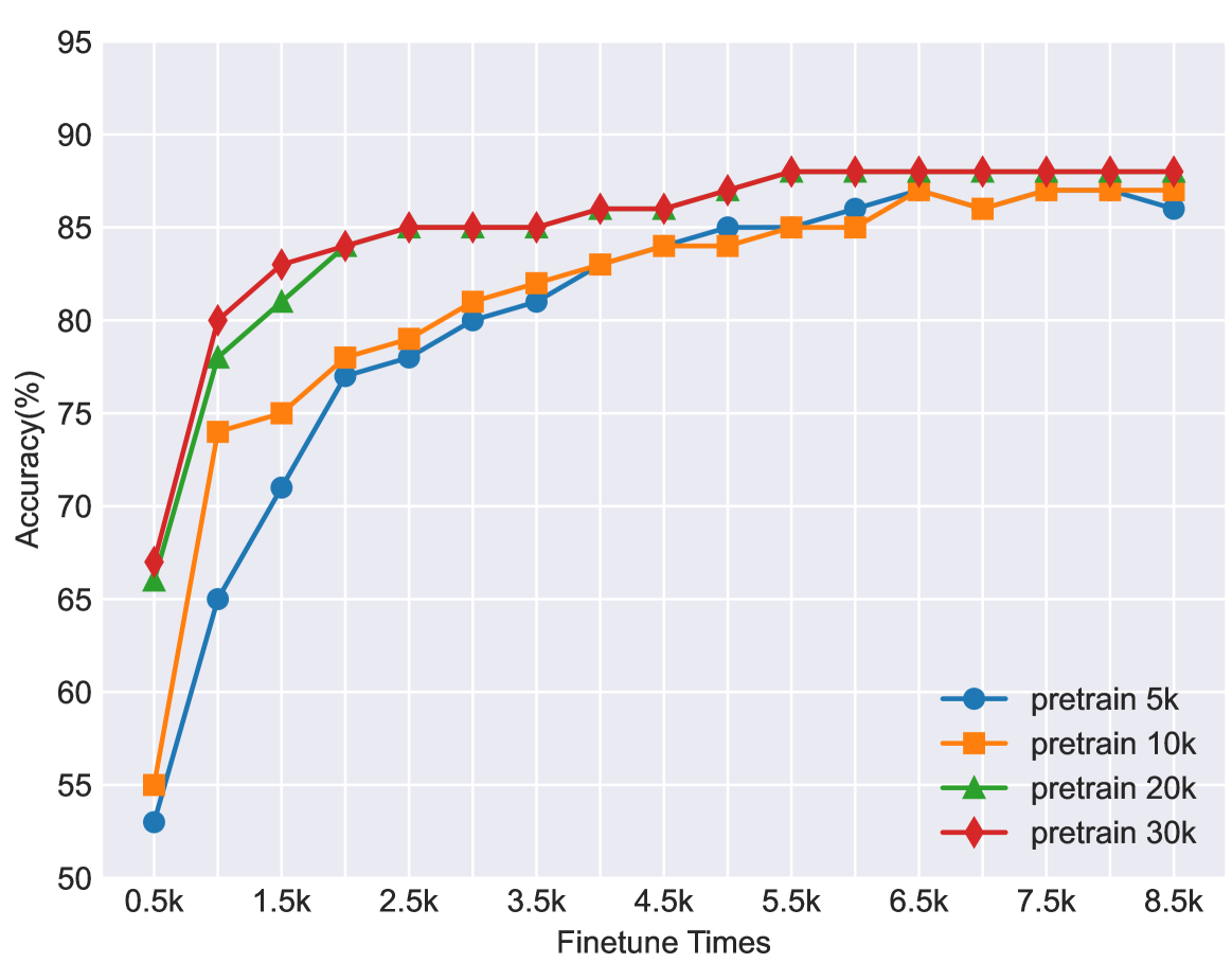
Figure 2: Comparison of results with different pre-training steps. The number of pre-training steps in unsupervised learning significantly impacts accuracy and fine-tuning convergence. In our experiments, pre-training for 30⁢K 30 𝐾 30K 30 italic_K steps achieved the best classification accuracy and the quickest convergence.

7 CONCLUSION

This paper presents a robust approach for the Keyword Spotting (KWS) task. Our CNN-Attention architecture, in combination with our unsupervised contrastive learning method, CABKS, utilizes unlabeled data efficiently. This circumvents the challenge of acquiring ample labeled training data, particularly beneficial when target keywords change or when positive samples are scarce. Furthermore, our speech augmentation strategy enhances the model’s robustness, adapting to variations in keyword utterances. By using contrastive loss within mini-batches, we’ve improved training efficiency and overall performance. Our method outperformed others such as CPC, APC, and MPC in experiments. Future work could explore this approach’s application to other speech tasks and investigate other augmentations or architectures to enhance performance. This work marks a significant step towards more reliable voice-controlled systems and interactive agents.

References

• [1] Chung, Y.A., Hsu, W.N., Tang, H., Glass, J.: An unsupervised autoregressive model for speech representation learning. arXiv preprint arXiv:1904.03240 (2019)
• [2] De Andrade, D.C., Leo, S., Viana, M.L.D.S., Bernkopf, C.: A neural attention model for speech command recognition. arXiv preprint arXiv:1808.08929 (2018)
• [3] Garcia, A., Gish, H.: Keyword spotting of arbitrary words using minimal speech resources. In: 2006 IEEE International Conference on Acoustics Speech and Signal Processing Proceedings. vol.1, pp.I–I. IEEE (2006)
• [4] Hannun, A., Case, C., Casper, J., Catanzaro, B., Diamos, G., Elsen, E., Prenger, R., Satheesh, S., Sengupta, S., Coates, A., et al.: Deep speech: Scaling up end-to-end speech recognition. arXiv preprint arXiv:1412.5567 (2014)
• [5] Jaitly, N., Hinton, G.E.: Vocal tract length perturbation (vtlp) improves speech recognition. In: Proc. ICML Workshop on Deep Learning for Audio, Speech and Language. vol.117, p.21 (2013)
• [6] Jiang, D., Lei, X., Li, W., Luo, N., Hu, Y., Zou, W., Li, X.: Improving transformer-based speech recognition using unsupervised pre-training. arXiv preprint arXiv:1910.09932 (2019)
• [7] Kharitonov, E., Rivière, M., Synnaeve, G., Wolf, L., Mazaré, P.E., Douze, M., Dupoux, E.: Data augmenting contrastive learning of speech representations in the time domain. In: 2021 IEEE Spoken Language Technology Workshop (SLT). pp. 215–222. IEEE (2021)
• [8] Ko, T., Peddinti, V., Povey, D., Khudanpur, S.: Audio augmentation for speech recognition. In: Sixteenth annual conference of the international speech communication association (2015)
• [9] Li, B., Sainath, T.N., Narayanan, A., Caroselli, J., Bacchiani, M., Misra, A., Shafran, I., Sak, H., Pundak, G., Chin, K.K., et al.: Acoustic modeling for google home. In: Interspeech. pp. 399–403 (2017)
• [10] Li, P., Liang, J., Xu, B.: A novel instance matching based unsupervised keyword spotting system. In: Second International Conference on Innovative Computing, Informatio and Control (ICICIC 2007). pp. 550–550. IEEE (2007)
• [11] Luo, J., Wang, J., Cheng, N., Jiang, G., Xiao, J.: End-to-end silent speech recognition with acoustic sensing. In: 2021 IEEE Spoken Language Technology Workshop (SLT). pp. 606–612. IEEE (2021)
• [12] Majumdar, S., Ginsburg, B.: Matchboxnet: 1d time-channel separable convolutional neural network architecture for speech commands recognition. arXiv preprint arXiv:2004.08531 (2020)
• [13] Oord, A.v.d., Li, Y., Vinyals, O.: Representation learning with contrastive predictive coding. arXiv preprint arXiv:1807.03748 (2018)
• [14] Panayotov, V., Chen, G., Povey, D., Khudanpur, S.: Librispeech: an asr corpus based on public domain audio books. In: 2015 IEEE international conference on acoustics, speech and signal processing (ICASSP). pp. 5206–5210. IEEE (2015)
• [15] Park, D.S., Chan, W., Zhang, Y., Chiu, C.C., Zoph, B., Cubuk, E.D., Le, Q.V.: Specaugment: A simple data augmentation method for automatic speech recognition. arXiv preprint arXiv:1904.08779 (2019)
• [16] Park, D.S., Zhang, Y., Jia, Y., Han, W., Chiu, C.C., Li, B., Wu, Y., Le, Q.V.: Improved noisy student training for automatic speech recognition. arXiv preprint arXiv:2005.09629 (2020)
• [17] Park, H.J., Zhu, P., Moreno, I.L., Subrahmanya, N.: Noisy student-teacher training for robust keyword spotting. arXiv preprint arXiv:2106.01604 (2021)
• [18] Schalkwyk, J., Beeferman, D., Beaufays, F., Byrne, B., Chelba, C., Cohen, M., Kamvar, M., Strope, B.: “your word is my command”: Google search by voice: A case study. Advances in Speech Recognition: Mobile Environments, Call Centers and Clinics pp. 61–90 (2010)
• [19] Tejedor, J., Toledano, D.T., Lopez-Otero, P., Docio-Fernandez, L., Peñagarikano, M., Rodriguez-Fuentes, L.J., Moreno-Sandoval, A.: Search on speech from spoken queries: the multi-domain international albayzin 2018 query-by-example spoken term detection evaluation. EURASIP Journal on Audio, Speech, and Music Processing 2019(1), 1–29 (2019)
• [20] Tejedor, J., Toledano, D.T., Lopez-Otero, P., Docio-Fernandez, L., Proença, J., Perdigão, F., García-Granada, F., Sanchis, E., Pompili, A., Abad, A.: Albayzin query-by-example spoken term detection 2016 evaluation. EURASIP Journal on Audio, Speech, and Music Processing 2018, 1–25 (2018)
• [21] Varol, G., Momeni, L., Albanie, S., Afouras, T., Zisserman, A.: Scaling up sign spotting through sign language dictionaries. International Journal of Computer Vision 130(6), 1416–1439 (2022)
• [22] Vygon, R., Mikhaylovskiy, N.: Learning efficient representations for keyword spotting with triplet loss. In: Speech and Computer: 23rd International Conference, SPECOM 2021, St. Petersburg, Russia, September 27–30, 2021, Proceedings 23. pp. 773–785. Springer (2021)
• [23] Warden, P.: Speech commands: A dataset for limited-vocabulary speech recognition. arXiv preprint arXiv:1804.03209 (2018)
• [24] Wei, Y., Gong, Z., Yang, S., Ye, K., Wen, Y.: Edgecrnn: an edge-computing oriented model of acoustic feature enhancement for keyword spotting. Journal of Ambient Intelligence and Humanized Computing pp. 1–11 (2022)
• [25] Zhang, Y., Glass, J.R.: Unsupervised spoken keyword spotting via segmental dtw on gaussian posteriorgrams. In: 2009 IEEE Workshop on Automatic Speech Recognition & Understanding. pp. 398–403. IEEE (2009)