2505/2505.00562.md

Title: TeLoGraF: Temporal Logic Planning via Graph-encoded Flow Matching

URL Source: https://arxiv.org/html/2505.00562

Markdown Content:

Abstract

Learning to solve complex tasks with signal temporal logic (STL) specifications is crucial to many real-world applications. However, most previous works only consider fixed or parametrized STL specifications due to the lack of a diverse STL dataset and encoders to effectively extract temporal logic information for downstream tasks. In this paper, we propose TeLoGraF, Te mporal Lo gic Gra ph-encoded F low, which utilizes Graph Neural Networks (GNN) encoder and flow-matching to learn solutions for general STL specifications. We identify four commonly used STL templates and collect a total of 200K specifications with paired demonstrations. We conduct extensive experiments in five simulation environments ranging from simple dynamical models in the 2D space to high-dimensional 7DoF Franka Panda robot arm and Ant quadruped navigation. Results show that our method outperforms other baselines in the STL satisfaction rate. Compared to classical STL planning algorithms, our approach is 10-100X faster in inference and can work on any system dynamics. Besides, we show our graph-encoding method’s capability to solve complex STLs and robustness to out-distribution STL specifications. Code is available at https://github.com/mengyuest/TeLoGraF.

Machine Learning, ICML

1 Introduction

Learning to plan for complex tasks with temporal dependency and logical constraints is critical to many real-world applications, such as navigation, autonomous vehicles, and industrial assembly lines. For example, a robot might need to reach one of the destination regions in 10 seconds while avoiding obstacles, a robot arm will need to pick the objects in a specific sequence, a vehicle should come to a complete stop before the stop sign and may proceed only if no other cars have the right of way, etc. These cases require precise reasoning and planning to ensure safety, efficiency, and correctness. Hence, it is of utmost importance to endow agents with the ability to tackle temporal logic constraints.

Existing temporal logic specifications can be mainly categorized into linear temporal logic (LTL)(Pnueli, 1977), computation tree logic (CTL)(Clarke & Emerson, 1981), metric temporal logic (MTL)(Koymans, 1990), and signal temporal logic (STL)(Donzé & Maler, 2010; Raman et al., 2015; He et al., 2022). LTL checks a single system trace via logical operators and temporal operators, whereas CTL reasons for a tree of possible futures. Extending from LTL, MTL introduces timed intervals for the temporal operators and STL further generalizes this by handling continuous-valued signals. In this work, we focus on STL since it offers the most expressive framework to handle a wide range of requirements in robotics and cyber-physical systems.

However, it is challenging to plan paths under STL specifications, due to its non-Markovian nature and lack of efficient decomposition. Synthesis for STL satisfaction is NP-hard(Kurtz & Lin, 2022). Classical methods for solving STL include sampling-based methods(Vasile et al., 2017; Kapoor et al., 2020), optimization-based methods(Sadraddini & Belta, 2015; Kurtz & Lin, 2022; Sun et al., 2022) and gradient-based methods(Dawson & Fan, 2022) but they cannot balance solution quality and computation efficiency for high-dimensional systems or complex STLs.

There is a growing trend to use learning-based methods to satisfy a given STL(Li et al., 2017; Puranic et al., 2021; Liu et al., 2021; Guo et al., 2024) or a family of parametrized STL(Leung & Pavone, 2022; Meng & Fan, 2024), but few of them can train one model to handle general STLs. If a new STL comes, they must retrain the neural network to learn the corresponding policy, resulting in inefficiency. Hashimoto et al. (2022) propose a model-based approach to handle flexible STL forms but requires differentiable environments. While other works(Zhong et al., 2023; Feng et al., 2024) explored regularizing the pre-trained models with temporal logic guidance at test time, the generated trajectories are heavily constrained by the original data distribution. To the best of our knowledge, there is no existing model that can take a general STL as input to produce satisfiable solutions.

Impeding the advance of STL-conditioned models are three critical challenges: (1) most of the papers either work on simplified STLs that are not diverse enough or useful but heavily engineer-designed STLs(Maierhofer et al., 2022; Meng & Fan, 2023) that are hard to generalize (2) there is no large-scale dataset available to provide paired demonstrations with diverse STL specifications and (3) unlike visual-conditioned or language-conditioned tasks, there lacks an analysis of the effective encoder design to embed the STL information to the downstream neural network.

In this paper, we tackle all these points above and propose TeLoGraF (Temporal Logic Graph-encoded Flow), a graph-encoded flow matching model that can handle general STL syntax and produce satisfiable trajectories. We first identify four commonly used STL templates and collect over 200K diverse STL specifications. We obtain paired demonstrations using off-the-shelf solvers under each robot domain. Finally, we argue that GNN is a suitable encoder to embed STL information for the downstream tasks and we systematically compare different encoder architectures for STL encoding over varied tasks.

Extensive experiments have been conducted over five simulation environments, ranging from simple linear and Dubins car dynamics in the 2D space, to high-dimensional Franka Panda robot arm and Ant quadruped maze navigation tasks. Compared to other encoder architectures, our GNN-based encoder can produce the highest quality solutions. Our method also outperforms other guidance-based imitation learning methods such as CTG(Zhong et al., 2023) and LTLDoG(Feng et al., 2024), demonstrating the need to bring STL into the training phase. Compared to classical methods (gradient-based(Dawson & Fan, 2022), CEM(Kapoor et al., 2020)), our approach is faster in inference and can work on any system dynamics and STL formats. Additional results also show our methods’ capability in handling complex STLs and out-distribution specifications.

Our contributions are as follows: (1) we are the first to learn a generative model for planning tasks conditioned on diverse STL specifications (2) we identify four key STL patterns and collect over 200K diverse STLs paired with demonstrations in five simulation environments (3) our proposed TeLoGraF demonstrates strong performance over other baselines and encoder architectures, which supports the design of using graph-encoding to extract different STLs (4) all the code and the datasets will be open-sourced to promote the development of STL planning.

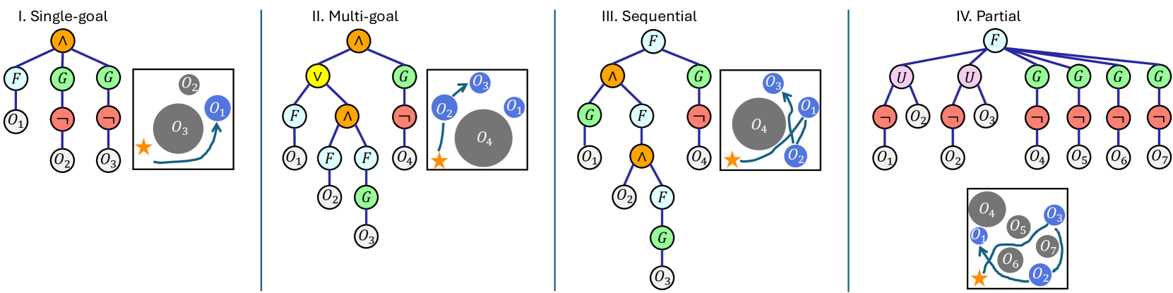
Figure 1: Four STL templates used in this paper. Single-goal: reach one goal under time constraints while avoiding obstacles. Multi-goal: reach one of the valid subsets of the goals. Sequential: All the goals needed to be reached in a strict temporal order. Partial: Some goals must be reached first before reaching other goals (no global order is explicitly specified).

2 Related work

Generative models for robotics. The rise of diffusion models in computer vision(Ho et al., 2020) has drawn massive attention in the robotic community. We refer the readers to this survey(Urain et al., 2024) for a full review. The general paradigm is to collect demonstrations from real-world(Chi et al., 2023; Zhong et al., 2023) or off-the-shelf solvers(Yang et al., 2023; Carvalho et al., 2023; Huang et al., 2024), and then train the neural network to imitate the data. Based on the input modality, the related works can be summarized into state-based(Janner et al., 2022), 2D diffusion policy(Chi et al., 2023), 3D diffusion policy(Ze et al., 2024; Ke et al., 2024), and vision language action models(Team et al., 2024). Varied output forms have been proposed, such as configuration-based(Yang et al., 2023), action-based(Chi et al., 2023; Ze et al., 2024), trajectory-based(Carvalho et al., 2023; Meng & Fan, 2024), and hierarchical models(Li et al., 2023; Chen et al., 2024). Regarding long-horizon task planning, compositional diffusion has been studied in GSC(Mishra et al., 2023) ChainedDiffuser(Xian et al., 2023) and DiMSam(Fang et al., 2024), where the task skeletons are usually fixed. More recently, flow-based methods(Chang et al., 2022; Chen et al., 2023; Prasad et al., 2024; Zhang et al., 2024) appear to have more stable training and faster sampling speed than diffusion models. Hence, we decide to use the linear flow discussed in(Liu et al., 2022) as our generative model backbone.

Signal Temporal Logic. Decades of efforts have been devoted to controlling robots under temporal and logical constraints(Fainekos et al., 2009; Wongpiromsarn et al., 2012). Unlike linear temporal logic(Finucane et al., 2010), STL is not equipped with a well-form automaton hence special treatment is needed for planning. Previous works include sampling-based method(Vasile et al., 2017), mixed-integer programming (MILP)(Sadraddini & Belta, 2015; Sun et al., 2022), evolutionary algorithms(Kapoor et al., 2020), gradient-based method(Dawson & Fan, 2022; Leung et al., 2023), reinforcement learning(Li et al., 2017) and model-based learning(Liu et al., 2021; Meng & Fan, 2023; Eappen et al., 2025). Temporal logic has been used to guide the diffusion models sampling in CTG(Zhong et al., 2023) for STL and in LTLDoG(Feng et al., 2024) for LTL, but they do not incorporate STL syntax during the training. Meng & Fan (2024) handles diverse STL in training but is limited to continuous parameters, whereas ours emphasizes handling general STL structures. The most similar to ours is Hashimoto et al. (2022), which studies different STL encoder architectures for model-based learning, but they work on shorter and simpler specifications without obstacles.

3 Preliminaries

3.1 Signal Temporal Logic (STL)

Consider a discrete-time system x t+1=f⁢(x t,u t)subscript 𝑥 𝑡 1 𝑓 subscript 𝑥 𝑡 subscript 𝑢 𝑡 x_{t+1}=f(x_{t},u_{t})italic_x start_POSTSUBSCRIPT italic_t + 1 end_POSTSUBSCRIPT = italic_f ( italic_x start_POSTSUBSCRIPT italic_t end_POSTSUBSCRIPT , italic_u start_POSTSUBSCRIPT italic_t end_POSTSUBSCRIPT ) where x t∈ℝ n subscript 𝑥 𝑡 superscript ℝ 𝑛 x_{t}\in\mathbb{R}^{n}italic_x start_POSTSUBSCRIPT italic_t end_POSTSUBSCRIPT ∈ blackboard_R start_POSTSUPERSCRIPT italic_n end_POSTSUPERSCRIPT is the state, and u t∈ℝ m subscript 𝑢 𝑡 superscript ℝ 𝑚 u_{t}\in\mathbb{R}^{m}italic_u start_POSTSUBSCRIPT italic_t end_POSTSUBSCRIPT ∈ blackboard_R start_POSTSUPERSCRIPT italic_m end_POSTSUPERSCRIPT is the control. Starting from an initial state x 0 subscript 𝑥 0 x_{0}italic_x start_POSTSUBSCRIPT 0 end_POSTSUBSCRIPT, a signal s=x 0,x 1,…,x T 𝑠 subscript 𝑥 0 subscript 𝑥 1…subscript 𝑥 𝑇 s=x_{0},x_{1},...,x_{T}italic_s = italic_x start_POSTSUBSCRIPT 0 end_POSTSUBSCRIPT , italic_x start_POSTSUBSCRIPT 1 end_POSTSUBSCRIPT , … , italic_x start_POSTSUBSCRIPT italic_T end_POSTSUBSCRIPT is generated via controls u 0,…,u T−1 subscript 𝑢 0…subscript 𝑢 𝑇 1 u_{0},...,u_{T-1}italic_u start_POSTSUBSCRIPT 0 end_POSTSUBSCRIPT , … , italic_u start_POSTSUBSCRIPT italic_T - 1 end_POSTSUBSCRIPT. STL specifies signal properties via the following rules(Donzé et al., 2013):

ϕ::=⊤|μ(x)≥0|¬ϕ|ϕ 1∧ϕ 2|ϕ 1 U[a,b]ϕ 2.\phi::=\top\ |\ \mu(x)\geq 0\ |\ \neg\phi\ |\ \phi_{1}\land\phi_{2}\ |\ \phi_{% 1}\text{U}{[a,b]}\phi{2}.italic_ϕ : := ⊤ | italic_μ ( italic_x ) ≥ 0 | ¬ italic_ϕ | italic_ϕ start_POSTSUBSCRIPT 1 end_POSTSUBSCRIPT ∧ italic_ϕ start_POSTSUBSCRIPT 2 end_POSTSUBSCRIPT | italic_ϕ start_POSTSUBSCRIPT 1 end_POSTSUBSCRIPT U start_POSTSUBSCRIPT [ italic_a , italic_b ] end_POSTSUBSCRIPT italic_ϕ start_POSTSUBSCRIPT 2 end_POSTSUBSCRIPT .(1)

Here the boolean-type operators split by “||||” are the building blocks to compose an STL: ⊤top\top⊤ means “true”, μ 𝜇\mu italic_μ denotes a function ℝ n→ℝ→superscript ℝ 𝑛 ℝ\mathbb{R}^{n}\to\mathbb{R}blackboard_R start_POSTSUPERSCRIPT italic_n end_POSTSUPERSCRIPT → blackboard_R, and ¬\neg¬, ∧\land∧, U, [a,b] are “not”, “and”, “until” and the time interval from a 𝑎 a italic_a to b 𝑏 b italic_b. Other operators are “or”: ϕ 1∨ϕ 2=¬(¬ϕ 1∧¬ϕ 2)subscript italic-ϕ 1 subscript italic-ϕ 2 subscript italic-ϕ 1 subscript italic-ϕ 2\phi_{1}\lor\phi_{2}=\neg(\neg\phi_{1}\land\neg\phi_{2})italic_ϕ start_POSTSUBSCRIPT 1 end_POSTSUBSCRIPT ∨ italic_ϕ start_POSTSUBSCRIPT 2 end_POSTSUBSCRIPT = ¬ ( ¬ italic_ϕ start_POSTSUBSCRIPT 1 end_POSTSUBSCRIPT ∧ ¬ italic_ϕ start_POSTSUBSCRIPT 2 end_POSTSUBSCRIPT ), “eventually”: ◆[a,b]⁢ϕ=⊤U[a,b]⁢ϕ subscript◆𝑎 𝑏 italic-ϕ top subscript U 𝑎 𝑏 italic-ϕ\lozenge_{[a,b]}\phi=\top\text{U}{[a,b]}\phi◆ start_POSTSUBSCRIPT [ italic_a , italic_b ] end_POSTSUBSCRIPT italic_ϕ = ⊤ U start_POSTSUBSCRIPT [ italic_a , italic_b ] end_POSTSUBSCRIPT italic_ϕ and “always”: □[a,b]⁢ϕ=¬◆[a,b]⁢¬ϕ subscript□𝑎 𝑏 italic-ϕ subscript◆𝑎 𝑏 italic-ϕ\square{[a,b]}\phi=\neg\lozenge_{[a,b]}\neg\phi□ start_POSTSUBSCRIPT [ italic_a , italic_b ] end_POSTSUBSCRIPT italic_ϕ = ¬ ◆ start_POSTSUBSCRIPT [ italic_a , italic_b ] end_POSTSUBSCRIPT ¬ italic_ϕ. We denote s,t⊧ϕ models 𝑠 𝑡 italic-ϕ s,t\models\phi italic_s , italic_t ⊧ italic_ϕ if the signal s 𝑠 s italic_s from time t 𝑡 t italic_t satisfies the STL formula (the evaluation of ϕ italic-ϕ\phi italic_ϕ returns True). For operators ⊤,μ>0,¬,∧formulae-sequence top 𝜇 0\top,\mu>0,\neg,\land⊤ , italic_μ > 0 , ¬ , ∧ and ∨\lor∨, the evaluation checks for the signal state at time t 𝑡 t italic_t. As for temporal operators(Maler & Nickovic, 2004): s,t⊧◆[a,b]⁢ϕ⇔∃t′∈[t+a,t+b]⁢s,t′⊧ϕ⇔models 𝑠 𝑡 subscript◆𝑎 𝑏 italic-ϕ formulae-sequence superscript 𝑡′𝑡 𝑎 𝑡 𝑏 𝑠 models superscript 𝑡′italic-ϕ s,t\models\lozenge_{[a,b]}\phi\Leftrightarrow,,\exists t^{\prime}\in[t+a,t+b% ],,s,t^{\prime}\models\phi italic_s , italic_t ⊧ ◆ start_POSTSUBSCRIPT [ italic_a , italic_b ] end_POSTSUBSCRIPT italic_ϕ ⇔ ∃ italic_t start_POSTSUPERSCRIPT ′ end_POSTSUPERSCRIPT ∈ [ italic_t + italic_a , italic_t + italic_b ] italic_s , italic_t start_POSTSUPERSCRIPT ′ end_POSTSUPERSCRIPT ⊧ italic_ϕ; and s,t⊧□[a,b]⁢ϕ⇔∀t′∈[t+a,t+b]⁢s,t′⊧ϕ⇔models 𝑠 𝑡 subscript□𝑎 𝑏 italic-ϕ formulae-sequence for-all superscript 𝑡′𝑡 𝑎 𝑡 𝑏 𝑠 models superscript 𝑡′italic-ϕ s,t\models\square_{[a,b]}\phi\Leftrightarrow,,\forall t^{\prime}\in[t+a,t+b]% ,,s,t^{\prime}\models\phi italic_s , italic_t ⊧ □ start_POSTSUBSCRIPT [ italic_a , italic_b ] end_POSTSUBSCRIPT italic_ϕ ⇔ ∀ italic_t start_POSTSUPERSCRIPT ′ end_POSTSUPERSCRIPT ∈ [ italic_t + italic_a , italic_t + italic_b ] italic_s , italic_t start_POSTSUPERSCRIPT ′ end_POSTSUPERSCRIPT ⊧ italic_ϕ; and s,t⊧ϕ 1⁢U[a,b]⁢ϕ 2⇔∃t′∈[t+a,t+b],s,t′⊧ϕ 2,∀t′′∈[0,t′],x,t′′⊧ϕ 1⇔models 𝑠 𝑡 subscript italic-ϕ 1 subscript 𝑈 𝑎 𝑏 subscript italic-ϕ 2 formulae-sequence superscript 𝑡′𝑡 𝑎 𝑡 𝑏 𝑠 formulae-sequence models superscript 𝑡′subscript italic-ϕ 2 formulae-sequence for-all superscript 𝑡′′0 superscript 𝑡′𝑥 models superscript 𝑡′′subscript italic-ϕ 1 s,t\models\phi_{1}U_{[a,b]}\phi_{2}\Leftrightarrow\exists t^{\prime}\in[t+a,t+% b],s,t^{\prime}\models\phi_{2},\forall t^{\prime\prime}\in[0,t^{\prime}],x,t^{% \prime\prime}\models\phi_{1}italic_s , italic_t ⊧ italic_ϕ start_POSTSUBSCRIPT 1 end_POSTSUBSCRIPT italic_U start_POSTSUBSCRIPT [ italic_a , italic_b ] end_POSTSUBSCRIPT italic_ϕ start_POSTSUBSCRIPT 2 end_POSTSUBSCRIPT ⇔ ∃ italic_t start_POSTSUPERSCRIPT ′ end_POSTSUPERSCRIPT ∈ [ italic_t + italic_a , italic_t + italic_b ] , italic_s , italic_t start_POSTSUPERSCRIPT ′ end_POSTSUPERSCRIPT ⊧ italic_ϕ start_POSTSUBSCRIPT 2 end_POSTSUBSCRIPT , ∀ italic_t start_POSTSUPERSCRIPT ′ ′ end_POSTSUPERSCRIPT ∈ [ 0 , italic_t start_POSTSUPERSCRIPT ′ end_POSTSUPERSCRIPT ] , italic_x , italic_t start_POSTSUPERSCRIPT ′ ′ end_POSTSUPERSCRIPT ⊧ italic_ϕ start_POSTSUBSCRIPT 1 end_POSTSUBSCRIPT. In plain words, ϕ 1⁢U[a,b]⁢ϕ 2 subscript italic-ϕ 1 subscript 𝑈 𝑎 𝑏 subscript italic-ϕ 2\phi_{1}U_{[a,b]}\phi_{2}italic_ϕ start_POSTSUBSCRIPT 1 end_POSTSUBSCRIPT italic_U start_POSTSUBSCRIPT [ italic_a , italic_b ] end_POSTSUBSCRIPT italic_ϕ start_POSTSUBSCRIPT 2 end_POSTSUBSCRIPT means “always hold ϕ 1 subscript italic-ϕ 1\phi_{1}italic_ϕ start_POSTSUBSCRIPT 1 end_POSTSUBSCRIPT true until ϕ 2 subscript italic-ϕ 2\phi_{2}italic_ϕ start_POSTSUBSCRIPT 2 end_POSTSUBSCRIPT happens in [a,b]𝑎 𝑏[a,b][ italic_a , italic_b ].” Robustness score(Donzé & Maler, 2010)ρ⁢(s,t,ϕ)𝜌 𝑠 𝑡 italic-ϕ\rho(s,t,\phi)italic_ρ ( italic_s , italic_t , italic_ϕ ) measures how well a signal s 𝑠 s italic_s satisfies ϕ italic-ϕ\phi italic_ϕ, where ρ≥0⁢iff⁢s,t⊧ϕ formulae-sequence 𝜌 0 iff 𝑠 models 𝑡 italic-ϕ\rho\geq 0\text{ iff }s,t\models\phi italic_ρ ≥ 0 iff italic_s , italic_t ⊧ italic_ϕ. The score is computed as:

ρ⁢(s,t,⊤)=1,ρ⁢(s,t,μ)=μ⁢(s⁢(t))formulae-sequence 𝜌 𝑠 𝑡 top 1 𝜌 𝑠 𝑡 𝜇 𝜇 𝑠 𝑡\displaystyle\rho(s,t,\top)=1,\quad\rho(s,t,\mu)=\mu(s(t))italic_ρ ( italic_s , italic_t , ⊤ ) = 1 , italic_ρ ( italic_s , italic_t , italic_μ ) = italic_μ ( italic_s ( italic_t ) )(2) ρ⁢(s,t,¬ϕ)=−ρ⁢(s,t,ϕ)𝜌 𝑠 𝑡 italic-ϕ 𝜌 𝑠 𝑡 italic-ϕ\displaystyle\rho(s,t,\neg\phi)=-\rho(s,t,\phi)italic_ρ ( italic_s , italic_t , ¬ italic_ϕ ) = - italic_ρ ( italic_s , italic_t , italic_ϕ ) ρ⁢(s,t,ϕ 1∧ϕ 2)=min⁡{ρ⁢(s,t,ϕ 1),ρ⁢(s,t,ϕ 2)}𝜌 𝑠 𝑡 subscript italic-ϕ 1 subscript italic-ϕ 2 𝜌 𝑠 𝑡 subscript italic-ϕ 1 𝜌 𝑠 𝑡 subscript italic-ϕ 2\displaystyle\rho(s,t,\phi_{1}\land\phi_{2})=\min{\rho(s,t,\phi_{1}),\rho(s,t% ,\phi_{2})}italic_ρ ( italic_s , italic_t , italic_ϕ start_POSTSUBSCRIPT 1 end_POSTSUBSCRIPT ∧ italic_ϕ start_POSTSUBSCRIPT 2 end_POSTSUBSCRIPT ) = roman_min { italic_ρ ( italic_s , italic_t , italic_ϕ start_POSTSUBSCRIPT 1 end_POSTSUBSCRIPT ) , italic_ρ ( italic_s , italic_t , italic_ϕ start_POSTSUBSCRIPT 2 end_POSTSUBSCRIPT ) } ρ⁢(s,t,◆[a,b]⁢ϕ)=sup r∈[a,b]ρ⁢(s,t+r,ϕ)𝜌 𝑠 𝑡 subscript◆𝑎 𝑏 italic-ϕ subscript supremum 𝑟 𝑎 𝑏 𝜌 𝑠 𝑡 𝑟 italic-ϕ\displaystyle\rho(s,t,\lozenge_{[a,b]}\phi)=\sup\limits_{r\in[a,b]}\rho(s,t+r,\phi)italic_ρ ( italic_s , italic_t , ◆ start_POSTSUBSCRIPT [ italic_a , italic_b ] end_POSTSUBSCRIPT italic_ϕ ) = roman_sup start_POSTSUBSCRIPT italic_r ∈ [ italic_a , italic_b ] end_POSTSUBSCRIPT italic_ρ ( italic_s , italic_t + italic_r , italic_ϕ ) ρ⁢(s,t,□[a,b]⁢ϕ)=inf r∈[a,b]ρ⁢(s,t+r,ϕ)𝜌 𝑠 𝑡 subscript□𝑎 𝑏 italic-ϕ subscript infimum 𝑟 𝑎 𝑏 𝜌 𝑠 𝑡 𝑟 italic-ϕ\displaystyle\rho(s,t,\square_{[a,b]}\phi)=\inf\limits_{r\in[a,b]}\rho(s,t+r,\phi)italic_ρ ( italic_s , italic_t , □ start_POSTSUBSCRIPT [ italic_a , italic_b ] end_POSTSUBSCRIPT italic_ϕ ) = roman_inf start_POSTSUBSCRIPT italic_r ∈ [ italic_a , italic_b ] end_POSTSUBSCRIPT italic_ρ ( italic_s , italic_t + italic_r , italic_ϕ ) ρ⁢(s,t,ϕ 1⁢U[a,b]⁢ϕ 2)=𝜌 𝑠 𝑡 subscript italic-ϕ 1 subscript U 𝑎 𝑏 subscript italic-ϕ 2 absent\displaystyle\rho(s,t,\phi_{1}\text{U}{[a,b]}\phi{2})=italic_ρ ( italic_s , italic_t , italic_ϕ start_POSTSUBSCRIPT 1 end_POSTSUBSCRIPT U start_POSTSUBSCRIPT [ italic_a , italic_b ] end_POSTSUBSCRIPT italic_ϕ start_POSTSUBSCRIPT 2 end_POSTSUBSCRIPT ) = sup t′∈[t+a,t+b]min⁡{ρ⁢(s,t′,ϕ 2),inf t′′∈[t,t′]ρ⁢(s,t′′,ϕ 1)}subscript supremum superscript 𝑡′𝑡 𝑎 𝑡 𝑏 𝜌 𝑠 superscript 𝑡′subscript italic-ϕ 2 subscript infimum superscript 𝑡′′𝑡 superscript 𝑡′𝜌 𝑠 superscript 𝑡′′subscript italic-ϕ 1\displaystyle\quad\sup\limits_{t^{\prime}\in[t+a,t+b]}\min\left{\rho(s,t^{% \prime},\phi_{2}),\inf\limits_{t^{\prime\prime}\in[t,t^{\prime}]}\rho(s,t^{% \prime\prime},\phi_{1})\right}roman_sup start_POSTSUBSCRIPT italic_t start_POSTSUPERSCRIPT ′ end_POSTSUPERSCRIPT ∈ [ italic_t + italic_a , italic_t + italic_b ] end_POSTSUBSCRIPT roman_min { italic_ρ ( italic_s , italic_t start_POSTSUPERSCRIPT ′ end_POSTSUPERSCRIPT , italic_ϕ start_POSTSUBSCRIPT 2 end_POSTSUBSCRIPT ) , roman_inf start_POSTSUBSCRIPT italic_t start_POSTSUPERSCRIPT ′ ′ end_POSTSUPERSCRIPT ∈ [ italic_t , italic_t start_POSTSUPERSCRIPT ′ end_POSTSUPERSCRIPT ] end_POSTSUBSCRIPT italic_ρ ( italic_s , italic_t start_POSTSUPERSCRIPT ′ ′ end_POSTSUPERSCRIPT , italic_ϕ start_POSTSUBSCRIPT 1 end_POSTSUBSCRIPT ) }

3.2 Diffusion models and flow matching

Diffusion models and flow matching learn a distribution from data samples. They both contain a forward process (for training) and an inverse process (for generating samples). For DDPM diffusion models(Ho et al., 2020), the data are diffused with Gaussian noise iteratively towards a white noise, and a neural network is trained to predict the noise at different diffusion steps. In the denoising process (inverse process), the samples initialized from the white noise are recovered gradually by removing the “noise” predicted by this neural net. For flow matching(Liu et al., 2022), in the forward process, the samples are continuously transformed into a Gaussian noise by a vector field, and the neural network learns to predict the vector field. During the inverse process, new samples are generated by integrating the predicted vector field over over time, starting from noise and progressively refining the samples.

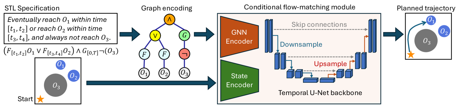
Figure 2: System diagram for TeLoGraF. The STL specification is encoded as a graph structure data. The GNN extracted embedding and the state embedding are sent to the Temporal U-Net flow model to generate the planned trajectory (via ODE).

4 Methodology

4.1 Problem formulation

Given a set of demonstrations 𝒟={(ϕ i,{τ i,k}k=1 K)}i=1 N 𝒟 superscript subscript subscript italic-ϕ 𝑖 superscript subscript subscript 𝜏 𝑖 𝑘 𝑘 1 𝐾 𝑖 1 𝑁\mathcal{D}={(\phi_{i},{\tau_{i,k}}{k=1}^{K})}{i=1}^{N}caligraphic_D = { ( italic_ϕ start_POSTSUBSCRIPT italic_i end_POSTSUBSCRIPT , { italic_τ start_POSTSUBSCRIPT italic_i , italic_k end_POSTSUBSCRIPT } start_POSTSUBSCRIPT italic_k = 1 end_POSTSUBSCRIPT start_POSTSUPERSCRIPT italic_K end_POSTSUPERSCRIPT ) } start_POSTSUBSCRIPT italic_i = 1 end_POSTSUBSCRIPT start_POSTSUPERSCRIPT italic_N end_POSTSUPERSCRIPT where ϕ i subscript italic-ϕ 𝑖\phi_{i}italic_ϕ start_POSTSUBSCRIPT italic_i end_POSTSUBSCRIPT is the STL formula defined in Sec.3.1, and {τ i,k}k=1 K superscript subscript subscript 𝜏 𝑖 𝑘 𝑘 1 𝐾{\tau_{i,k}}{k=1}^{K}{ italic_τ start_POSTSUBSCRIPT italic_i , italic_k end_POSTSUBSCRIPT } start_POSTSUBSCRIPT italic_k = 1 end_POSTSUBSCRIPT start_POSTSUPERSCRIPT italic_K end_POSTSUPERSCRIPT is a batch of trajectories that satisfy the STL specification, ∀k,τ i,k,0⊧ϕ i models for-all 𝑘 subscript 𝜏 𝑖 𝑘 0 subscript italic-ϕ 𝑖\forall k,\tau{i,k},0\models\phi_{i}∀ italic_k , italic_τ start_POSTSUBSCRIPT italic_i , italic_k end_POSTSUBSCRIPT , 0 ⊧ italic_ϕ start_POSTSUBSCRIPT italic_i end_POSTSUBSCRIPT, our goal is to learn a conditional generative model p θ⁢(τ|x 0,ϕ)subscript 𝑝 𝜃 conditional 𝜏 subscript 𝑥 0 italic-ϕ p_{\theta}(\tau|x_{0},\phi)italic_p start_POSTSUBSCRIPT italic_θ end_POSTSUBSCRIPT ( italic_τ | italic_x start_POSTSUBSCRIPT 0 end_POSTSUBSCRIPT , italic_ϕ ), so that given a query STL specification ϕ italic-ϕ\phi italic_ϕ and an initial state x 0 subscript 𝑥 0 x_{0}italic_x start_POSTSUBSCRIPT 0 end_POSTSUBSCRIPT, the trajectories sampled from this learned distribution τ∼p θ(⋅|ϕ,x 0)\tau\sim p_{\theta}(\cdot|\phi,x_{0})italic_τ ∼ italic_p start_POSTSUBSCRIPT italic_θ end_POSTSUBSCRIPT ( ⋅ | italic_ϕ , italic_x start_POSTSUBSCRIPT 0 end_POSTSUBSCRIPT ) can satisfy the STL specification, i.e., τ,0⊧ϕ models 𝜏 0 italic-ϕ\tau,0\models\phi italic_τ , 0 ⊧ italic_ϕ.

4.2 STL specification templates

We aim to collect specifications that are both general and representative of the unique characteristics of the STL. Since our focus is primarily on addressing the complexity of STL rather than the skills required to perform each subtask, we restrict the set of atomic propositions semantics to “reach” (an object / a region) and “avoid” (an object / a region), while excluding operations that involve dexterity or agility skills. We want to emphasize the “temporal” and the “logical” facets of the STL specifications, where the former includes both absolute time constraints or relative temporal ordering (dependencies), and the latter captures patterns to describe multi-choice and selections. In this paper, we consider four types of STL templates: single-goal, multi-goal, sequential, and partial-order, denoted as ϕ s⁢i⁢n⁢g⁢l⁢e subscript italic-ϕ 𝑠 𝑖 𝑛 𝑔 𝑙 𝑒\phi_{single}italic_ϕ start_POSTSUBSCRIPT italic_s italic_i italic_n italic_g italic_l italic_e end_POSTSUBSCRIPT, ϕ m⁢u⁢l⁢t⁢i subscript italic-ϕ 𝑚 𝑢 𝑙 𝑡 𝑖\phi_{multi}italic_ϕ start_POSTSUBSCRIPT italic_m italic_u italic_l italic_t italic_i end_POSTSUBSCRIPT, ϕ s⁢e⁢q⁢u⁢e⁢n⁢t⁢i⁢a⁢l subscript italic-ϕ 𝑠 𝑒 𝑞 𝑢 𝑒 𝑛 𝑡 𝑖 𝑎 𝑙\phi_{sequential}italic_ϕ start_POSTSUBSCRIPT italic_s italic_e italic_q italic_u italic_e italic_n italic_t italic_i italic_a italic_l end_POSTSUBSCRIPT, and ϕ p⁢a⁢r⁢t⁢i⁢a⁢l subscript italic-ϕ 𝑝 𝑎 𝑟 𝑡 𝑖 𝑎 𝑙\phi_{partial}italic_ϕ start_POSTSUBSCRIPT italic_p italic_a italic_r italic_t italic_i italic_a italic_l end_POSTSUBSCRIPT in the following Backus-Naur Form (BNF) (similar to Sec.3.1, the symbols on the left-hand side of “::=:absent assign::=: :=” can take any of the forms split by “||||” shown on the right-hand side of the expression):

ϕ r⁢e⁢a⁢c⁢h::=:subscript italic-ϕ 𝑟 𝑒 𝑎 𝑐 ℎ assign\displaystyle\phi_{reach}::=italic_ϕ start_POSTSUBSCRIPT italic_r italic_e italic_a italic_c italic_h end_POSTSUBSCRIPT : :=F[t a,t b]O|F[t a,t b]G[t c,t d]O\displaystyle F_{[t_{a},t_{b}]}O\ \ |\ \ F_{[t_{a},t_{b}]}G_{[t_{c},t_{d}]}O italic_F start_POSTSUBSCRIPT [ italic_t start_POSTSUBSCRIPT italic_a end_POSTSUBSCRIPT , italic_t start_POSTSUBSCRIPT italic_b end_POSTSUBSCRIPT ] end_POSTSUBSCRIPT italic_O | italic_F start_POSTSUBSCRIPT [ italic_t start_POSTSUBSCRIPT italic_a end_POSTSUBSCRIPT , italic_t start_POSTSUBSCRIPT italic_b end_POSTSUBSCRIPT ] end_POSTSUBSCRIPT italic_G start_POSTSUBSCRIPT [ italic_t start_POSTSUBSCRIPT italic_c end_POSTSUBSCRIPT , italic_t start_POSTSUBSCRIPT italic_d end_POSTSUBSCRIPT ] end_POSTSUBSCRIPT italic_O(3) ϕ a⁢v⁢o⁢i⁢d::=:subscript italic-ϕ 𝑎 𝑣 𝑜 𝑖 𝑑 assign\displaystyle\phi_{avoid}::=italic_ϕ start_POSTSUBSCRIPT italic_a italic_v italic_o italic_i italic_d end_POSTSUBSCRIPT : :=⊤|G[0,T]¬O|ϕ a⁢v⁢o⁢i⁢d,1∧ϕ a⁢v⁢o⁢i⁢d,2\displaystyle\top\ \ |\ \ G_{[0,T]}\neg O\ \ |\ \ \phi_{avoid,1}\land\phi_{% avoid,2}⊤ | italic_G start_POSTSUBSCRIPT [ 0 , italic_T ] end_POSTSUBSCRIPT ¬ italic_O | italic_ϕ start_POSTSUBSCRIPT italic_a italic_v italic_o italic_i italic_d , 1 end_POSTSUBSCRIPT ∧ italic_ϕ start_POSTSUBSCRIPT italic_a italic_v italic_o italic_i italic_d , 2 end_POSTSUBSCRIPT ϕ a⁢n⁢d::=:subscript italic-ϕ 𝑎 𝑛 𝑑 assign\displaystyle\phi_{and}::=italic_ϕ start_POSTSUBSCRIPT italic_a italic_n italic_d end_POSTSUBSCRIPT : :=⋀i=1 n 1 ϕ r⁢e⁢a⁢c⁢h,i⁢⋀j=1 n 2(ϕ o⁢r,j)superscript subscript 𝑖 1 subscript 𝑛 1 subscript italic-ϕ 𝑟 𝑒 𝑎 𝑐 ℎ 𝑖 superscript subscript 𝑗 1 subscript 𝑛 2 subscript italic-ϕ 𝑜 𝑟 𝑗\displaystyle\bigwedge_{i=1}^{n_{1}}\phi_{reach,i}\bigwedge_{j=1}^{n_{2}}\left% (\phi_{or,j}\right)⋀ start_POSTSUBSCRIPT italic_i = 1 end_POSTSUBSCRIPT start_POSTSUPERSCRIPT italic_n start_POSTSUBSCRIPT 1 end_POSTSUBSCRIPT end_POSTSUPERSCRIPT italic_ϕ start_POSTSUBSCRIPT italic_r italic_e italic_a italic_c italic_h , italic_i end_POSTSUBSCRIPT ⋀ start_POSTSUBSCRIPT italic_j = 1 end_POSTSUBSCRIPT start_POSTSUPERSCRIPT italic_n start_POSTSUBSCRIPT 2 end_POSTSUBSCRIPT end_POSTSUPERSCRIPT ( italic_ϕ start_POSTSUBSCRIPT italic_o italic_r , italic_j end_POSTSUBSCRIPT ) ϕ o⁢r::=:subscript italic-ϕ 𝑜 𝑟 assign\displaystyle\phi_{or}::=italic_ϕ start_POSTSUBSCRIPT italic_o italic_r end_POSTSUBSCRIPT : :=⋁i=1 n 1 ϕ r⁢e⁢a⁢c⁢h,i⁢⋁j=1 n 2(ϕ a⁢n⁢d,j)superscript subscript 𝑖 1 subscript 𝑛 1 subscript italic-ϕ 𝑟 𝑒 𝑎 𝑐 ℎ 𝑖 superscript subscript 𝑗 1 subscript 𝑛 2 subscript italic-ϕ 𝑎 𝑛 𝑑 𝑗\displaystyle\bigvee_{i=1}^{n_{1}}\phi_{reach,i}\bigvee_{j=1}^{n_{2}}\left(% \phi_{and,j}\right)⋁ start_POSTSUBSCRIPT italic_i = 1 end_POSTSUBSCRIPT start_POSTSUPERSCRIPT italic_n start_POSTSUBSCRIPT 1 end_POSTSUBSCRIPT end_POSTSUPERSCRIPT italic_ϕ start_POSTSUBSCRIPT italic_r italic_e italic_a italic_c italic_h , italic_i end_POSTSUBSCRIPT ⋁ start_POSTSUBSCRIPT italic_j = 1 end_POSTSUBSCRIPT start_POSTSUPERSCRIPT italic_n start_POSTSUBSCRIPT 2 end_POSTSUBSCRIPT end_POSTSUPERSCRIPT ( italic_ϕ start_POSTSUBSCRIPT italic_a italic_n italic_d , italic_j end_POSTSUBSCRIPT ) ϕ s⁢i⁢n⁢g⁢l⁢e::=:subscript italic-ϕ 𝑠 𝑖 𝑛 𝑔 𝑙 𝑒 assign\displaystyle\phi_{single}::=italic_ϕ start_POSTSUBSCRIPT italic_s italic_i italic_n italic_g italic_l italic_e end_POSTSUBSCRIPT : :=ϕ r⁢e⁢a⁢c⁢h∧ϕ a⁢v⁢o⁢i⁢d subscript italic-ϕ 𝑟 𝑒 𝑎 𝑐 ℎ subscript italic-ϕ 𝑎 𝑣 𝑜 𝑖 𝑑\displaystyle\phi_{reach}\land\phi_{avoid}italic_ϕ start_POSTSUBSCRIPT italic_r italic_e italic_a italic_c italic_h end_POSTSUBSCRIPT ∧ italic_ϕ start_POSTSUBSCRIPT italic_a italic_v italic_o italic_i italic_d end_POSTSUBSCRIPT ϕ m⁢u⁢l⁢t⁢i::=:subscript italic-ϕ 𝑚 𝑢 𝑙 𝑡 𝑖 assign\displaystyle\phi_{multi}::=italic_ϕ start_POSTSUBSCRIPT italic_m italic_u italic_l italic_t italic_i end_POSTSUBSCRIPT : :=ϕ a⁢n⁢d∧ϕ a⁢v⁢o⁢i⁢d|ϕ o⁢r\displaystyle\phi_{and}\land\phi_{avoid}\ \ |\ \ \phi_{or}italic_ϕ start_POSTSUBSCRIPT italic_a italic_n italic_d end_POSTSUBSCRIPT ∧ italic_ϕ start_POSTSUBSCRIPT italic_a italic_v italic_o italic_i italic_d end_POSTSUBSCRIPT | italic_ϕ start_POSTSUBSCRIPT italic_o italic_r end_POSTSUBSCRIPT ϕ s⁢e⁢q⁢u⁢e⁢n⁢t⁢i⁢a⁢l::=:subscript italic-ϕ 𝑠 𝑒 𝑞 𝑢 𝑒 𝑛 𝑡 𝑖 𝑎 𝑙 assign\displaystyle\phi_{sequential}::=italic_ϕ start_POSTSUBSCRIPT italic_s italic_e italic_q italic_u italic_e italic_n italic_t italic_i italic_a italic_l end_POSTSUBSCRIPT : :=ϕ r⁢e⁢a⁢c⁢h|F[t a,t b](O∧ϕ s⁢e⁢q⁢u⁢e⁢n⁢t⁢i⁢a⁢l)∧ϕ a⁢v⁢o⁢i⁢d\displaystyle\phi_{reach}\ \ |\ \ F_{[t_{a},t_{b}]}(O\land\phi_{sequential})% \land\phi_{avoid}italic_ϕ start_POSTSUBSCRIPT italic_r italic_e italic_a italic_c italic_h end_POSTSUBSCRIPT | italic_F start_POSTSUBSCRIPT [ italic_t start_POSTSUBSCRIPT italic_a end_POSTSUBSCRIPT , italic_t start_POSTSUBSCRIPT italic_b end_POSTSUBSCRIPT ] end_POSTSUBSCRIPT ( italic_O ∧ italic_ϕ start_POSTSUBSCRIPT italic_s italic_e italic_q italic_u italic_e italic_n italic_t italic_i italic_a italic_l end_POSTSUBSCRIPT ) ∧ italic_ϕ start_POSTSUBSCRIPT italic_a italic_v italic_o italic_i italic_d end_POSTSUBSCRIPT ϕ p⁢a⁢r⁢t⁢i⁢a⁢l::=:subscript italic-ϕ 𝑝 𝑎 𝑟 𝑡 𝑖 𝑎 𝑙 assign\displaystyle\phi_{partial}::=italic_ϕ start_POSTSUBSCRIPT italic_p italic_a italic_r italic_t italic_i italic_a italic_l end_POSTSUBSCRIPT : :=⋀i=1 n 1¬O p i⁢U[0,T]⁢O q i∧⋀j=1 n 2 ϕ r⁢e⁢a⁢c⁢h,r j∧ϕ a⁢v⁢o⁢i⁢d superscript subscript 𝑖 1 subscript 𝑛 1 subscript 𝑂 subscript 𝑝 𝑖 subscript 𝑈 0 𝑇 subscript 𝑂 subscript 𝑞 𝑖 superscript subscript 𝑗 1 subscript 𝑛 2 subscript italic-ϕ 𝑟 𝑒 𝑎 𝑐 ℎ subscript 𝑟 𝑗 subscript italic-ϕ 𝑎 𝑣 𝑜 𝑖 𝑑\displaystyle\bigwedge_{i=1}^{n_{1}}\neg O_{p_{i}}U_{[0,T]}O_{q_{i}}\land% \bigwedge_{j=1}^{n_{2}}\phi_{reach,r_{j}}\land\phi_{avoid}⋀ start_POSTSUBSCRIPT italic_i = 1 end_POSTSUBSCRIPT start_POSTSUPERSCRIPT italic_n start_POSTSUBSCRIPT 1 end_POSTSUBSCRIPT end_POSTSUPERSCRIPT ¬ italic_O start_POSTSUBSCRIPT italic_p start_POSTSUBSCRIPT italic_i end_POSTSUBSCRIPT end_POSTSUBSCRIPT italic_U start_POSTSUBSCRIPT [ 0 , italic_T ] end_POSTSUBSCRIPT italic_O start_POSTSUBSCRIPT italic_q start_POSTSUBSCRIPT italic_i end_POSTSUBSCRIPT end_POSTSUBSCRIPT ∧ ⋀ start_POSTSUBSCRIPT italic_j = 1 end_POSTSUBSCRIPT start_POSTSUPERSCRIPT italic_n start_POSTSUBSCRIPT 2 end_POSTSUBSCRIPT end_POSTSUPERSCRIPT italic_ϕ start_POSTSUBSCRIPT italic_r italic_e italic_a italic_c italic_h , italic_r start_POSTSUBSCRIPT italic_j end_POSTSUBSCRIPT end_POSTSUBSCRIPT ∧ italic_ϕ start_POSTSUBSCRIPT italic_a italic_v italic_o italic_i italic_d end_POSTSUBSCRIPT

where O i subscript 𝑂 𝑖 O_{i}italic_O start_POSTSUBSCRIPT italic_i end_POSTSUBSCRIPT is the atomic proposition representing “reach the i 𝑖 i italic_i-th object”, and ¬O 𝑂\neg O¬ italic_O means “avoid the object”. ϕ r⁢e⁢a⁢c⁢h subscript italic-ϕ 𝑟 𝑒 𝑎 𝑐 ℎ\phi_{reach}italic_ϕ start_POSTSUBSCRIPT italic_r italic_e italic_a italic_c italic_h end_POSTSUBSCRIPT means “eventually reach the object at time interval [t a,t b]subscript 𝑡 𝑎 subscript 𝑡 𝑏[t_{a},t_{b}][ italic_t start_POSTSUBSCRIPT italic_a end_POSTSUBSCRIPT , italic_t start_POSTSUBSCRIPT italic_b end_POSTSUBSCRIPT ] (and stay there for the time interval [t a+t c,t b+t d]subscript 𝑡 𝑎 subscript 𝑡 𝑐 subscript 𝑡 𝑏 subscript 𝑡 𝑑[t_{a}+t_{c},t_{b}+t_{d}][ italic_t start_POSTSUBSCRIPT italic_a end_POSTSUBSCRIPT + italic_t start_POSTSUBSCRIPT italic_c end_POSTSUBSCRIPT , italic_t start_POSTSUBSCRIPT italic_b end_POSTSUBSCRIPT + italic_t start_POSTSUBSCRIPT italic_d end_POSTSUBSCRIPT ] if G[t c,t d]subscript 𝐺 subscript 𝑡 𝑐 subscript 𝑡 𝑑 G_{[t_{c},t_{d}]}italic_G start_POSTSUBSCRIPT [ italic_t start_POSTSUBSCRIPT italic_c end_POSTSUBSCRIPT , italic_t start_POSTSUBSCRIPT italic_d end_POSTSUBSCRIPT ] end_POSTSUBSCRIPT is specified)”. ϕ a⁢v⁢o⁢i⁢d subscript italic-ϕ 𝑎 𝑣 𝑜 𝑖 𝑑\phi_{avoid}italic_ϕ start_POSTSUBSCRIPT italic_a italic_v italic_o italic_i italic_d end_POSTSUBSCRIPT means “always avoid obstacles for all time (here [0,T]0 𝑇[0,T][ 0 , italic_T ] denotes the full time horizon)”. ϕ a⁢n⁢d subscript italic-ϕ 𝑎 𝑛 𝑑\phi_{and}italic_ϕ start_POSTSUBSCRIPT italic_a italic_n italic_d end_POSTSUBSCRIPT and ϕ o⁢r subscript italic-ϕ 𝑜 𝑟\phi_{or}italic_ϕ start_POSTSUBSCRIPT italic_o italic_r end_POSTSUBSCRIPT mean “reach a subset of objects” (for example, ϕ r⁢e⁢a⁢c⁢h,1∨(ϕ r⁢e⁢a⁢c⁢h,2∧ϕ r⁢e⁢a⁢c⁢h,3)subscript italic-ϕ 𝑟 𝑒 𝑎 𝑐 ℎ 1 subscript italic-ϕ 𝑟 𝑒 𝑎 𝑐 ℎ 2 subscript italic-ϕ 𝑟 𝑒 𝑎 𝑐 ℎ 3\phi_{reach,1}\lor\left(\phi_{reach,2}\land\phi_{reach,3}\right)italic_ϕ start_POSTSUBSCRIPT italic_r italic_e italic_a italic_c italic_h , 1 end_POSTSUBSCRIPT ∨ ( italic_ϕ start_POSTSUBSCRIPT italic_r italic_e italic_a italic_c italic_h , 2 end_POSTSUBSCRIPT ∧ italic_ϕ start_POSTSUBSCRIPT italic_r italic_e italic_a italic_c italic_h , 3 end_POSTSUBSCRIPT ) means “reach O 1 subscript 𝑂 1 O_{1}italic_O start_POSTSUBSCRIPT 1 end_POSTSUBSCRIPT or reach both O 2 subscript 𝑂 2 O_{2}italic_O start_POSTSUBSCRIPT 2 end_POSTSUBSCRIPT and O 3 subscript 𝑂 3 O_{3}italic_O start_POSTSUBSCRIPT 3 end_POSTSUBSCRIPT”).

A graphical illustration for the examples can be found in Figure.1. The template ϕ s⁢i⁢n⁢g⁢l⁢e subscript italic-ϕ 𝑠 𝑖 𝑛 𝑔 𝑙 𝑒\phi_{single}italic_ϕ start_POSTSUBSCRIPT italic_s italic_i italic_n italic_g italic_l italic_e end_POSTSUBSCRIPT specifies the single-goal-reaching with time constraints. The template ϕ m⁢u⁢l⁢t⁢i subscript italic-ϕ 𝑚 𝑢 𝑙 𝑡 𝑖\phi_{multi}italic_ϕ start_POSTSUBSCRIPT italic_m italic_u italic_l italic_t italic_i end_POSTSUBSCRIPT specifies a subset of goals to reach. The third template ϕ s⁢e⁢q⁢u⁢e⁢n⁢t⁢i⁢a⁢l subscript italic-ϕ 𝑠 𝑒 𝑞 𝑢 𝑒 𝑛 𝑡 𝑖 𝑎 𝑙\phi_{sequential}italic_ϕ start_POSTSUBSCRIPT italic_s italic_e italic_q italic_u italic_e italic_n italic_t italic_i italic_a italic_l end_POSTSUBSCRIPT specifies multiple goals that must be reached in a specific order. And the last template ϕ p⁢a⁢r⁢t⁢i⁢a⁢l subscript italic-ϕ 𝑝 𝑎 𝑟 𝑡 𝑖 𝑎 𝑙\phi_{partial}italic_ϕ start_POSTSUBSCRIPT italic_p italic_a italic_r italic_t italic_i italic_a italic_l end_POSTSUBSCRIPT specifies some objects (O p i subscript 𝑂 subscript 𝑝 𝑖 O_{p_{i}}italic_O start_POSTSUBSCRIPT italic_p start_POSTSUBSCRIPT italic_i end_POSTSUBSCRIPT end_POSTSUBSCRIPT) need to be reached after other objects (O q i subscript 𝑂 subscript 𝑞 𝑖 O_{q_{i}}italic_O start_POSTSUBSCRIPT italic_q start_POSTSUBSCRIPT italic_i end_POSTSUBSCRIPT end_POSTSUBSCRIPT) are reached, and some objects needed to be reached within time constraints (O r j subscript 𝑂 subscript 𝑟 𝑗 O_{r_{j}}italic_O start_POSTSUBSCRIPT italic_r start_POSTSUBSCRIPT italic_j end_POSTSUBSCRIPT end_POSTSUBSCRIPT). All the templates are further paired with ϕ a⁢v⁢o⁢i⁢d subscript italic-ϕ 𝑎 𝑣 𝑜 𝑖 𝑑\phi_{avoid}italic_ϕ start_POSTSUBSCRIPT italic_a italic_v italic_o italic_i italic_d end_POSTSUBSCRIPT to reflect safety constraints.

(a)Linear

(b)Dubins

(c)PointMaze

(d)AntMaze

(e)Franka Panda

Figure 3: Simulation benchmarks. In Linear and Dubins, a moving robot needs to reach circular regions and avoid circular obstacles. In PointMaze and AntMaze, the agent needs to reach/avoid square tiles in a maze. In Franka Panda, the robot arm needs to reach certain cubes on the table while not colliding with red balls.

4.3 Encoder design

To capture the information from an STL, we treat the STL as a syntax tree, and create a graph node for every operator and atomic proposition node in the syntax tree. The graph nodes are connected based on the edges on the syntax tree, where for every connection, we use a directed edge pointing from the child node to its father node. Mathmatically, given an STL syntax tree, we represent it as a directed graph 1 1 1 Here, we overload the symbol G 𝐺 G italic_G previously used as the “always” operator for consistency with the normal notation.G=(V,E,H)∈𝒢 𝐺 𝑉 𝐸 𝐻 𝒢 G=(V,E,H)\in\mathcal{G}italic_G = ( italic_V , italic_E , italic_H ) ∈ caligraphic_G with nodes set V 𝑉 V italic_V, edge set E 𝐸 E italic_E and node features H 𝐻 H italic_H (edges pointing from the child node to its father node), where each node feature h v∈ℝ d G subscript ℎ 𝑣 superscript ℝ subscript 𝑑 𝐺 h_{v}\in\mathbb{R}^{d_{G}}italic_h start_POSTSUBSCRIPT italic_v end_POSTSUBSCRIPT ∈ blackboard_R start_POSTSUPERSCRIPT italic_d start_POSTSUBSCRIPT italic_G end_POSTSUBSCRIPT end_POSTSUPERSCRIPT contains all the attributes to characterize an STL operator or atomic proposition (AP), including the operator type I t⁢y⁢p⁢e∈ℤ subscript 𝐼 𝑡 𝑦 𝑝 𝑒 ℤ I_{type}\in\mathbb{Z}italic_I start_POSTSUBSCRIPT italic_t italic_y italic_p italic_e end_POSTSUBSCRIPT ∈ blackboard_Z, start time and end time t s⁢t⁢a⁢r⁢t,t e⁢n⁢d∈0,…,T formulae-sequence subscript 𝑡 𝑠 𝑡 𝑎 𝑟 𝑡 subscript 𝑡 𝑒 𝑛 𝑑 0…𝑇 t_{start},t_{end}\in 0,...,T italic_t start_POSTSUBSCRIPT italic_s italic_t italic_a italic_r italic_t end_POSTSUBSCRIPT , italic_t start_POSTSUBSCRIPT italic_e italic_n italic_d end_POSTSUBSCRIPT ∈ 0 , … , italic_T (for operators and APs that do not have the time intervals, we use -1 as the default value), object coordinates x,y,z 𝑥 𝑦 𝑧 x,y,z italic_x , italic_y , italic_z and radius r 𝑟 r italic_r (or side length, depending on whether the object is a circle/sphere or a square/cube). Besides, for the Until operator, we need to distinguish its left child with its right child as the order matters, so we use a separate binary variable to indicate whether it is the left child of the Until operator. In total, the node feature dimension is d G=8 subscript 𝑑 𝐺 8 d_{G}=8 italic_d start_POSTSUBSCRIPT italic_G end_POSTSUBSCRIPT = 8.

A multi-layer GNN ℱ θ:𝒢→ℝ d z:subscript ℱ 𝜃→𝒢 superscript ℝ subscript 𝑑 𝑧\mathcal{F}{\theta}:\mathcal{G}\to\mathbb{R}^{d{z}}caligraphic_F start_POSTSUBSCRIPT italic_θ end_POSTSUBSCRIPT : caligraphic_G → blackboard_R start_POSTSUPERSCRIPT italic_d start_POSTSUBSCRIPT italic_z end_POSTSUBSCRIPT end_POSTSUPERSCRIPT operates on this graph data G 𝐺 G italic_G to get a d z subscript 𝑑 𝑧 d_{z}italic_d start_POSTSUBSCRIPT italic_z end_POSTSUBSCRIPT-dimension embedding. It first iteratively updates the node representations through message passing. The initial node feature for the node v 𝑣 v italic_v is h v(0)=h v superscript subscript ℎ 𝑣 0 subscript ℎ 𝑣 h_{v}^{(0)}=h_{v}italic_h start_POSTSUBSCRIPT italic_v end_POSTSUBSCRIPT start_POSTSUPERSCRIPT ( 0 ) end_POSTSUPERSCRIPT = italic_h start_POSTSUBSCRIPT italic_v end_POSTSUBSCRIPT discussed above. At each layer l 𝑙 l italic_l of the GNN, the node v 𝑣 v italic_v’s feature h v(l)superscript subscript ℎ 𝑣 𝑙 h_{v}^{(l)}italic_h start_POSTSUBSCRIPT italic_v end_POSTSUBSCRIPT start_POSTSUPERSCRIPT ( italic_l ) end_POSTSUPERSCRIPT is updated based on the message passing procedure with its neighbors (children) 𝒩⁢(v)𝒩 𝑣\mathcal{N}(v)caligraphic_N ( italic_v ):

h v(l+1)=γ⁢(h v(l),⊕u∈𝒩⁢(v)ψ⁢(h v(l),h u(l)))superscript subscript ℎ 𝑣 𝑙 1 𝛾 superscript subscript ℎ 𝑣 𝑙 subscript direct-sum 𝑢 𝒩 𝑣 𝜓 superscript subscript ℎ 𝑣 𝑙 superscript subscript ℎ 𝑢 𝑙 h_{v}^{(l+1)}=\gamma\left(h_{v}^{(l)},\mathop{\oplus}\limits_{u\in\mathcal{N}(% v)}\psi(h_{v}^{(l)},h_{u}^{(l)})\right)italic_h start_POSTSUBSCRIPT italic_v end_POSTSUBSCRIPT start_POSTSUPERSCRIPT ( italic_l + 1 ) end_POSTSUPERSCRIPT = italic_γ ( italic_h start_POSTSUBSCRIPT italic_v end_POSTSUBSCRIPT start_POSTSUPERSCRIPT ( italic_l ) end_POSTSUPERSCRIPT , ⊕ start_POSTSUBSCRIPT italic_u ∈ caligraphic_N ( italic_v ) end_POSTSUBSCRIPT italic_ψ ( italic_h start_POSTSUBSCRIPT italic_v end_POSTSUBSCRIPT start_POSTSUPERSCRIPT ( italic_l ) end_POSTSUPERSCRIPT , italic_h start_POSTSUBSCRIPT italic_u end_POSTSUBSCRIPT start_POSTSUPERSCRIPT ( italic_l ) end_POSTSUPERSCRIPT ) )(4)

here γ(.)\gamma(.)italic_γ ( . ) and ψ 𝜓\psi italic_ψ are the nonlinear update and message functions to increase the expressiveness of the GNN, and ⊕direct-sum\oplus⊕ is the permutation-invariant function (e.g., sum, mean, min, max). After L 𝐿 L italic_L layers of message passing, the final representation h v(L)∈ℝ d z superscript subscript ℎ 𝑣 𝐿 superscript ℝ subscript 𝑑 𝑧 h_{v}^{(L)}\in\mathbb{R}^{d_{z}}italic_h start_POSTSUBSCRIPT italic_v end_POSTSUBSCRIPT start_POSTSUPERSCRIPT ( italic_L ) end_POSTSUPERSCRIPT ∈ blackboard_R start_POSTSUPERSCRIPT italic_d start_POSTSUBSCRIPT italic_z end_POSTSUBSCRIPT end_POSTSUPERSCRIPT is read out using another aggregation function h G=⊕v∈V h v(L)subscript ℎ 𝐺 subscript direct-sum 𝑣 𝑉 superscript subscript ℎ 𝑣 𝐿 h_{G}=\mathop{\oplus}\limits_{v\in V}h_{v}^{(L)}italic_h start_POSTSUBSCRIPT italic_G end_POSTSUBSCRIPT = ⊕ start_POSTSUBSCRIPT italic_v ∈ italic_V end_POSTSUBSCRIPT italic_h start_POSTSUBSCRIPT italic_v end_POSTSUBSCRIPT start_POSTSUPERSCRIPT ( italic_L ) end_POSTSUPERSCRIPT, which will be used for the downstream trajectory generation task.

4.4 Expressiveness of GNN to encode STL

It is crucial to verify theoretically that the GNN can distinguish different STLs. The work(Xu et al., 2018) shows GNN has (at most) the same expressiveness as the 1-dimensional Weisfeiler Leman graph isomorphism test (WL-test). It has been shown in(Kiefer, 2020) that the WL-test is a complete test for trees, hence GNN can distinguish two STLs (syntax trees) if they are different on the graph level.

4.5 Conditional flow for trajectory generation

Given the STL embedding z∈ℝ d z 𝑧 superscript ℝ subscript 𝑑 𝑧 z\in\mathbb{R}^{d_{z}}italic_z ∈ blackboard_R start_POSTSUPERSCRIPT italic_d start_POSTSUBSCRIPT italic_z end_POSTSUBSCRIPT end_POSTSUPERSCRIPT for ϕ italic-ϕ\phi italic_ϕ and the initial state x 0∈ℝ n subscript 𝑥 0 superscript ℝ 𝑛 x_{0}\in\mathbb{R}^{n}italic_x start_POSTSUBSCRIPT 0 end_POSTSUBSCRIPT ∈ blackboard_R start_POSTSUPERSCRIPT italic_n end_POSTSUPERSCRIPT, we aim to learn a conditional flow neural network ℋ ω:ℝ n×ℝ d z×ℝ 1×ℝ T×(m+n)→ℝ T×(m+n):subscript ℋ 𝜔→superscript ℝ 𝑛 superscript ℝ subscript 𝑑 𝑧 superscript ℝ 1 superscript ℝ 𝑇 𝑚 𝑛 superscript ℝ 𝑇 𝑚 𝑛\mathcal{H}{\omega}:\mathbb{R}^{n}\times\mathbb{R}^{d{z}}\times\mathbb{R}^{1% }\times\mathbb{R}^{T\times(m+n)}\to\mathbb{R}^{T\times(m+n)}caligraphic_H start_POSTSUBSCRIPT italic_ω end_POSTSUBSCRIPT : blackboard_R start_POSTSUPERSCRIPT italic_n end_POSTSUPERSCRIPT × blackboard_R start_POSTSUPERSCRIPT italic_d start_POSTSUBSCRIPT italic_z end_POSTSUBSCRIPT end_POSTSUPERSCRIPT × blackboard_R start_POSTSUPERSCRIPT 1 end_POSTSUPERSCRIPT × blackboard_R start_POSTSUPERSCRIPT italic_T × ( italic_m + italic_n ) end_POSTSUPERSCRIPT → blackboard_R start_POSTSUPERSCRIPT italic_T × ( italic_m + italic_n ) end_POSTSUPERSCRIPT to generate the trajectory τ^∈ℝ T×(m+n)^𝜏 superscript ℝ 𝑇 𝑚 𝑛\hat{\tau}\in\mathbb{R}^{T\times(m+n)}over^ start_ARG italic_τ end_ARG ∈ blackboard_R start_POSTSUPERSCRIPT italic_T × ( italic_m + italic_n ) end_POSTSUPERSCRIPT that can satisfy the STL. In each training step, we randomly draw a demonstration 2 2 2 We use X 0 subscript 𝑋 0 X_{0}italic_X start_POSTSUBSCRIPT 0 end_POSTSUBSCRIPT to denote the samples from the source distribution, and X 1 subscript 𝑋 1 X_{1}italic_X start_POSTSUBSCRIPT 1 end_POSTSUBSCRIPT for the samples from the target data distribution, while using x 𝑥 x italic_x for the states in the trajectory.X 1=τ subscript 𝑋 1 𝜏 X_{1}=\tau italic_X start_POSTSUBSCRIPT 1 end_POSTSUBSCRIPT = italic_τ with its corresponding STL ϕ italic-ϕ\phi italic_ϕ from the dataset (x 0 subscript 𝑥 0 x_{0}italic_x start_POSTSUBSCRIPT 0 end_POSTSUBSCRIPT is the first state in τ 𝜏\tau italic_τ) and randomly draw X 0 subscript 𝑋 0 X_{0}italic_X start_POSTSUBSCRIPT 0 end_POSTSUBSCRIPT from the Gaussian distribution 𝒩⁢(0,I)𝒩 0 𝐼\mathcal{N}(0,I)caligraphic_N ( 0 , italic_I ) and denote Δ⁢X=X 1−X 0 Δ 𝑋 subscript 𝑋 1 subscript 𝑋 0\Delta X=X_{1}-X_{0}roman_Δ italic_X = italic_X start_POSTSUBSCRIPT 1 end_POSTSUBSCRIPT - italic_X start_POSTSUBSCRIPT 0 end_POSTSUBSCRIPT. Then, we uniformly sample t∼Uniform⁢(0,1)similar-to 𝑡 Uniform 0 1 t\sim\text{Uniform}(0,1)italic_t ∼ Uniform ( 0 , 1 ) and take the linear combination: X t=t⁢X 1+(1−t)⁢X 0 subscript 𝑋 𝑡 𝑡 subscript 𝑋 1 1 𝑡 subscript 𝑋 0 X_{t}=tX_{1}+(1-t)X_{0}italic_X start_POSTSUBSCRIPT italic_t end_POSTSUBSCRIPT = italic_t italic_X start_POSTSUBSCRIPT 1 end_POSTSUBSCRIPT + ( 1 - italic_t ) italic_X start_POSTSUBSCRIPT 0 end_POSTSUBSCRIPT. We denote G 𝐺 G italic_G as the graph for ϕ italic-ϕ\phi italic_ϕ as mentioned in Sec.4.3. To this end, we can formulate the Flow Matching loss:

ℒ F⁢M=𝔼 t,X 0,X 1⁢‖ℋ ω⁢(ℱ θ⁢(G),x 0,t,X t)−Δ⁢X‖2 subscript ℒ 𝐹 𝑀 subscript 𝔼 𝑡 subscript 𝑋 0 subscript 𝑋 1 superscript norm subscript ℋ 𝜔 subscript ℱ 𝜃 𝐺 subscript 𝑥 0 𝑡 subscript 𝑋 𝑡 Δ 𝑋 2\mathcal{L}{FM}=\mathbb{E}{t,X_{0},X_{1}}||\mathcal{H}{\omega}\left(% \mathcal{F}{\theta}(G),x_{0},t,X_{t}\right)-\Delta X||^{2}caligraphic_L start_POSTSUBSCRIPT italic_F italic_M end_POSTSUBSCRIPT = blackboard_E start_POSTSUBSCRIPT italic_t , italic_X start_POSTSUBSCRIPT 0 end_POSTSUBSCRIPT , italic_X start_POSTSUBSCRIPT 1 end_POSTSUBSCRIPT end_POSTSUBSCRIPT | | caligraphic_H start_POSTSUBSCRIPT italic_ω end_POSTSUBSCRIPT ( caligraphic_F start_POSTSUBSCRIPT italic_θ end_POSTSUBSCRIPT ( italic_G ) , italic_x start_POSTSUBSCRIPT 0 end_POSTSUBSCRIPT , italic_t , italic_X start_POSTSUBSCRIPT italic_t end_POSTSUBSCRIPT ) - roman_Δ italic_X | | start_POSTSUPERSCRIPT 2 end_POSTSUPERSCRIPT(5)

which is used to update the neural network parameters θ 𝜃\theta italic_θ and ω 𝜔\omega italic_ω in the training. The network ℋ ω subscript ℋ 𝜔\mathcal{H}{\omega}caligraphic_H start_POSTSUBSCRIPT italic_ω end_POSTSUBSCRIPT learns a velocity field (conditional on ϕ italic-ϕ\phi italic_ϕ and x 0 subscript 𝑥 0 x{0}italic_x start_POSTSUBSCRIPT 0 end_POSTSUBSCRIPT) which determines a flow ψ:[0,1]×ℝ T×(m+n)→ℝ T×(m+n):𝜓→0 1 superscript ℝ 𝑇 𝑚 𝑛 superscript ℝ 𝑇 𝑚 𝑛\psi:[0,1]\times\mathbb{R}^{T\times(m+n)}\to\mathbb{R}^{T\times(m+n)}italic_ψ : [ 0 , 1 ] × blackboard_R start_POSTSUPERSCRIPT italic_T × ( italic_m + italic_n ) end_POSTSUPERSCRIPT → blackboard_R start_POSTSUPERSCRIPT italic_T × ( italic_m + italic_n ) end_POSTSUPERSCRIPT, depicted as d d⁢t⁢ψ⁢(t,X)=ℋ ω⁢(ℱ θ⁢(G),x 0,t,ψ⁢(t,X))𝑑 𝑑 𝑡 𝜓 𝑡 𝑋 subscript ℋ 𝜔 subscript ℱ 𝜃 𝐺 subscript 𝑥 0 𝑡 𝜓 𝑡 𝑋\quad\frac{d}{dt}\psi(t,X)=\mathcal{H}{\omega}(\mathcal{F}{\theta}(G),x_{0},% t,\psi(t,X))divide start_ARG italic_d end_ARG start_ARG italic_d italic_t end_ARG italic_ψ ( italic_t , italic_X ) = caligraphic_H start_POSTSUBSCRIPT italic_ω end_POSTSUBSCRIPT ( caligraphic_F start_POSTSUBSCRIPT italic_θ end_POSTSUBSCRIPT ( italic_G ) , italic_x start_POSTSUBSCRIPT 0 end_POSTSUBSCRIPT , italic_t , italic_ψ ( italic_t , italic_X ) ) with initial condition ψ⁢(0,X)=X 𝜓 0 𝑋 𝑋\psi(0,X)=X italic_ψ ( 0 , italic_X ) = italic_X. Therefore, we can generate the target sample by first randomly sampling X′∼𝒩⁢(0,I)similar-to superscript 𝑋′𝒩 0 𝐼 X^{\prime}\sim\mathcal{N}(0,I)italic_X start_POSTSUPERSCRIPT ′ end_POSTSUPERSCRIPT ∼ caligraphic_N ( 0 , italic_I ), then solve the ODE with X=X′,t=0 formulae-sequence 𝑋 superscript 𝑋′𝑡 0 X=X^{\prime},t=0 italic_X = italic_X start_POSTSUPERSCRIPT ′ end_POSTSUPERSCRIPT , italic_t = 0 until t=1 𝑡 1 t=1 italic_t = 1, and the target sample will be τ^=ψ⁢(1,X′)^𝜏 𝜓 1 superscript 𝑋′\hat{\tau}=\psi(1,X^{\prime})over^ start_ARG italic_τ end_ARG = italic_ψ ( 1 , italic_X start_POSTSUPERSCRIPT ′ end_POSTSUPERSCRIPT ). To solve ODE numerically, we discretize the ODE time domain into N s subscript 𝑁 𝑠 N_{s}italic_N start_POSTSUBSCRIPT italic_s end_POSTSUBSCRIPT steps, and sample t 𝑡 t italic_t uniformly from {0,1 N s,2 N s,…,1}0 1 subscript 𝑁 𝑠 2 subscript 𝑁 𝑠…1{0,\frac{1}{N_{s}},\frac{2}{N_{s}},...,1}{ 0 , divide start_ARG 1 end_ARG start_ARG italic_N start_POSTSUBSCRIPT italic_s end_POSTSUBSCRIPT end_ARG , divide start_ARG 2 end_ARG start_ARG italic_N start_POSTSUBSCRIPT italic_s end_POSTSUBSCRIPT end_ARG , … , 1 } in training. In testing, from random sample X′superscript 𝑋′X^{\prime}italic_X start_POSTSUPERSCRIPT ′ end_POSTSUPERSCRIPT, we run Euler’s method to solve ODE: ψ⁢(t i+1,X′)=ψ⁢(t i,X′)+ℋ ω⁢(ℱ θ⁢(G),x 0,t i,ψ⁢(t i,X′))N s 𝜓 subscript 𝑡 𝑖 1 superscript 𝑋′𝜓 subscript 𝑡 𝑖 superscript 𝑋′subscript ℋ 𝜔 subscript ℱ 𝜃 𝐺 subscript 𝑥 0 subscript 𝑡 𝑖 𝜓 subscript 𝑡 𝑖 superscript 𝑋′subscript 𝑁 𝑠\psi(t_{i+1},X^{\prime})=\psi(t_{i},X^{\prime})+\frac{\mathcal{H}{\omega}(% \mathcal{F}{\theta}(G),x_{0},t_{i},\psi(t_{i},X^{\prime}))}{N_{s}}italic_ψ ( italic_t start_POSTSUBSCRIPT italic_i + 1 end_POSTSUBSCRIPT , italic_X start_POSTSUPERSCRIPT ′ end_POSTSUPERSCRIPT ) = italic_ψ ( italic_t start_POSTSUBSCRIPT italic_i end_POSTSUBSCRIPT , italic_X start_POSTSUPERSCRIPT ′ end_POSTSUPERSCRIPT ) + divide start_ARG caligraphic_H start_POSTSUBSCRIPT italic_ω end_POSTSUBSCRIPT ( caligraphic_F start_POSTSUBSCRIPT italic_θ end_POSTSUBSCRIPT ( italic_G ) , italic_x start_POSTSUBSCRIPT 0 end_POSTSUBSCRIPT , italic_t start_POSTSUBSCRIPT italic_i end_POSTSUBSCRIPT , italic_ψ ( italic_t start_POSTSUBSCRIPT italic_i end_POSTSUBSCRIPT , italic_X start_POSTSUPERSCRIPT ′ end_POSTSUPERSCRIPT ) ) end_ARG start_ARG italic_N start_POSTSUBSCRIPT italic_s end_POSTSUBSCRIPT end_ARG, where t i=i N s,for i=0,1⁢…,N s−1 subscript 𝑡 𝑖 𝑖 subscript 𝑁 𝑠 for i=0,1⁢…,N s−1 t_{i}=\frac{i}{N_{s}},,\text{for $i=0,1...,N_{s}-1$}italic_t start_POSTSUBSCRIPT italic_i end_POSTSUBSCRIPT = divide start_ARG italic_i end_ARG start_ARG italic_N start_POSTSUBSCRIPT italic_s end_POSTSUBSCRIPT end_ARG , for italic_i = 0 , 1 … , italic_N start_POSTSUBSCRIPT italic_s end_POSTSUBSCRIPT - 1.

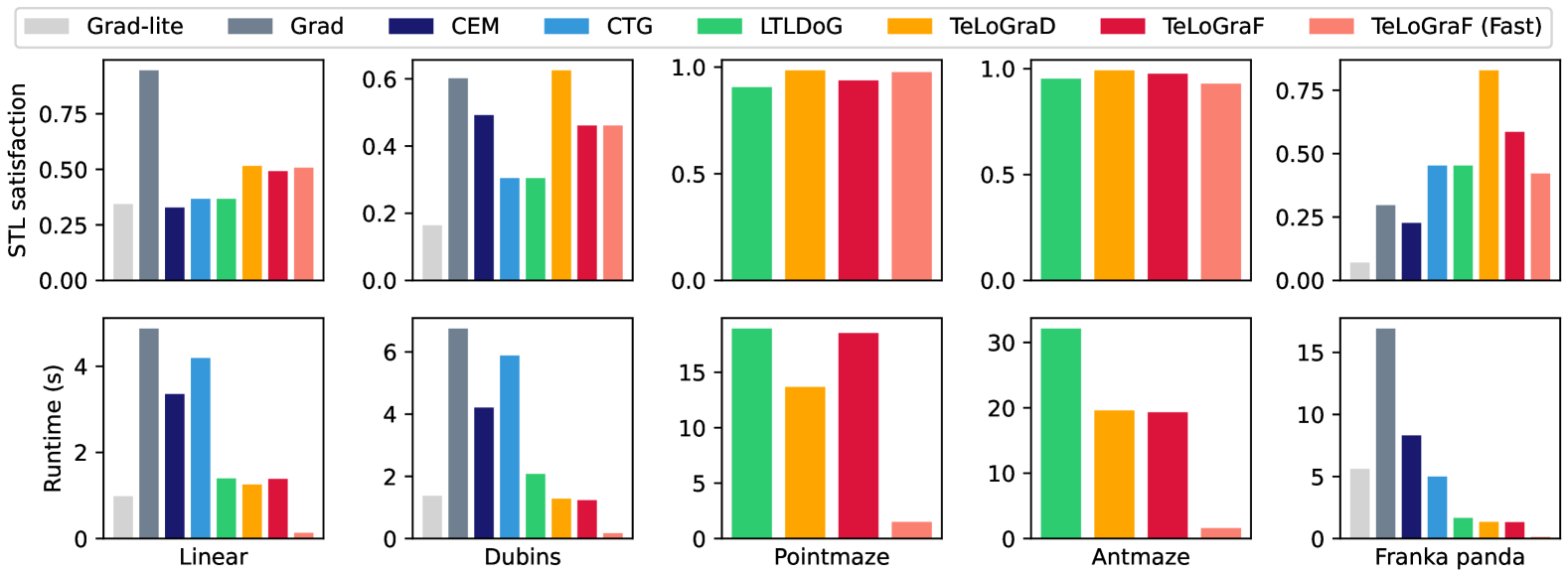
Figure 4: Main results. Our methods outperform both learning-based methods (CTG and LTLDoG) and classical methods (Grad, CEM). In four out of the five benchmarks, TeLoGraD achieves the highest solution quality. TeLoGraF (Fast) achieves the best trade-off between solution quality and efficiency over all benchmarks, especially being 123.6X faster than Grad and 60.7X faster than CEM with a higher satisfaction rate in the Franka Panda environment.

5 Experiments

Implementation details. We consider five robot simulation environments, including ZoneEnv in Jackermeier & Abate (2024) with Linear (single-integrator dynamics) and Dubins (Car dynamics), PointMaze, AntMaze(Fu et al., 2020) and Franka Panda robot arm(Gaz et al., 2019). The trajectory length is 512 for PointMaze and AntMaze and 64 for the other environments. For each robot domain, we start with the four STL templates discussed in Sec.4.2, and for each template, we randomly generate 10000 STL specifications with 2 to 12 objects (regions) for goals and obstacles, and randomly initialize the agent location in each case. For simulation environments like Linear/Dubins and Franka Panda, we use a gradient-based solver to collect trajectories that maximize the STL robustness scores. For non-differentiable environments like PointMaze and AntMaze, we first plan for waypoints on the grids using A* search algorithm, then we use waypoint tracking controllers to generate the low-level trajectories. For each STL, we generate 2 demonstrations, resulting in 80k trajectories under each robot domain. We use 80%percent 80 80%80 % for training and 20%percent 20 20%20 % for validation. Our TeLoGraF uses a GNN encoder with GCN layers(Kipf & Welling, 2016) with 4 hidden layers and 256 units in each layer, and a ReLU activation(Nair & Hinton, 2010) is used for the intermediate layers. The output embedding dimension is 256. The backbone network follows the UNet architecture used in(Janner et al., 2022) with two extra input for the STL embedding and the initial states. In the flow matching, we set the flow step N s=100 subscript 𝑁 𝑠 100 N_{s}=100 italic_N start_POSTSUBSCRIPT italic_s end_POSTSUBSCRIPT = 100. The learning pipeline is implemented in Pytorch Geometric(Fey & Lenssen, 2019; Paszke et al., 2019). The training is conducted for 1000 epochs with a batch size of 256. We use the commonly used ADAM(Kingma, 2014) optimizer with an initial learning rate 5×10−4 5 superscript 10 4 5\times 10^{-4}5 × 10 start_POSTSUPERSCRIPT - 4 end_POSTSUPERSCRIPT and a cosine annealing schedule that reduces the learning rate to 5×10−5 5 superscript 10 5 5\times 10^{-5}5 × 10 start_POSTSUPERSCRIPT - 5 end_POSTSUPERSCRIPT at the 900-th epochs and then keep it as constant for the rest 100 epochs. We use Nvidia L40S GPUs for the training, where each training job takes 6-24 hours on a single GPU. During evaluation, for each graph, we sample 256 STL specifications from the training and the validation sets for comparison.

Baselines. We compare with both classical and learning-based methods for STL specification planning. For the classical methods 3 3 3 We compare with classical methods only on selected differentiable environments., we compare with Grad: a gradient-based method in Dawson & Fan (2022), Grad-lite: using the gradient-based method but with fewer iterations, and CEM: a sampling-based method(Kapoor et al., 2020). For the learning-based baselines, we compare with CTG:(Zhong et al., 2023), which uses gradient guidance for the diffusion models, and LTLDoG:(Feng et al., 2024), which uses classifier guidance for the diffusion models (we change their LTL classifier to an STL classifier for our tasks). We also consider varied forms of encoder architectures, such as GRU:(Chung et al., 2014), which uses gated recurrent units to encode the sequence of STL formula, similar to Hashimoto et al. (2022), Transformer:(Vaswani, 2017), which uses attention-based auto-regressive models to encode the sequence of STL formula similar to GRU, and TreeLSTM:(Tai et al., 2015), which is similar to GNN but instead of synchronized message passing, TreeLSTM updates nodes features layer-by-layer via LSTM in a bottom-up fashion on syntax trees. Our method consists three variations, TeLoGraD (D iffusion): which uses GNN as encoder and learns the trajectories via diffusion models, TeLoGraF: which uses GNN as encoder and learns the trajectories via flow models, and TeLoGraF (Fast): uses the pretrained TeLoGraF model with less ODE steps to generate samples.

Metrics.. For each STL, we sample 1024 trajectories and pick the one with the highest STL score as the final trajectory. We compute the average STL satisfaction rate for the final trajectories (ratio of final trajectories that satisfy the STL) and the average computation runtime for the trajectory generation. Without special notice, we focused on the validation set STL satisfaction rate because the satisfaction rate in the training split is close to 1.

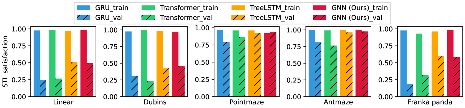
Figure 5: Different encoder architecture comparisons. GNN and TreeLSTM works the best on the validation set.

5.1 Main results

We first compare our method variations (TeLoGraD, TeLoGraF, and TeLoGraF (Fast)) with classical and learning-based STL planning baselines. As shown in Fig.4, on most of the environments, our methods achieve a better trade-off between solution quality and runtime. TeLoGraD achieves the highest performance regarding STL satisfaction, with the computation budget lower than almost all the baselines (except Grad-lite on Linear environment, but Grad-lite has low satisfaction rate), which first shows the efficacy of our designed pipeline. The advantage over classical methods increases as we move from low-dimension environments to the high-dimension Franka Panda environment, as both gradient-based and sampling-based methods struggles to provide high-quality solutions in a high-dimension space. Compared to learning-based methods such as CTG and LTLDoG, our methods do not compute the time-consuming guidance step in the inference stage, hence achieving better efficiency. Interestingly, the results under the maze environments (PointMaze and AntMaze) are very close among these learning-based methods, and the STL satisfaction rate is the highest among all environments. This is probably because the data distribution is limited to the maze layout, making learning easier. Among our methods, TeLoGraF and TeLoGraF(Fast) replace the diffusion models in TeLoGraD with flow-matching models, leading to a performance drop in Dubins and Franka Panda environments, which might be owed to the nonlinear dynamics or forward-kinematics under these environments. However, TeLoGraF (Fast) can achieve on par of TeLoGraF’s satisfaction rate with only 1/10 of the runtime, making itself a super-efficient algorithm. On Franka Panda environment, TeLoGraF (Fast) is 123.6X faster than Grad and 60.7X faster than CEM with a higher satisfaction rate than both methods. Overall, the results demonstrate that TeLoGraD provides the best balance between solution quality and computational efficiency, while TeLoGraF (Fast) emerges as a promising alternative for real-time applications for the temporal logic task planning.

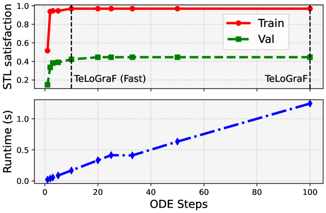
Figure 6: Ablation studies on ODE steps in Dubins environment. TeLoGraF(Fast) achieves a similar STL satisfaction compared to TeLoGraF with only 1/10 of its runtime.

5.2 Ablation study on the flow steps

To understand how fast the flow model can be accelerated while maintaining the solution quality, we design a test on the Dubins environment with varied number of flow steps for the sampling. The original TeLoGraF needs to run 100 ODE steps for data generation. Here, we reduce the ODE steps by increasing the ODE time step size 4 4 4 This ODE time step size should be distinguished with the algorithm runtime. The ODE time interval is fixed from 0 to 1 in the flow model sampling process. Thus, the step size in each ODE step determines the number of ODE steps needed. in each flow step. We evaluate the solution quality by checking its STL satisfaction. As shown in Fig.6, the algorithm runtime grows linearly with the number of ODE steps. The STL satisfaction rate for the original TeLoGraF is 0.97 on the training split and 0.45 on the validation split. The scores do not drop until the number of ODE steps decreases to 10. Even with 2 ODE steps, the model can obtain an STL satisfaction rate of 0.94 on the training split and 0.34 on the validation. These observations demonstrate the sampling efficiency of the flow models and we hence use 10 ODE steps for “TeLoGraF (fast)”.

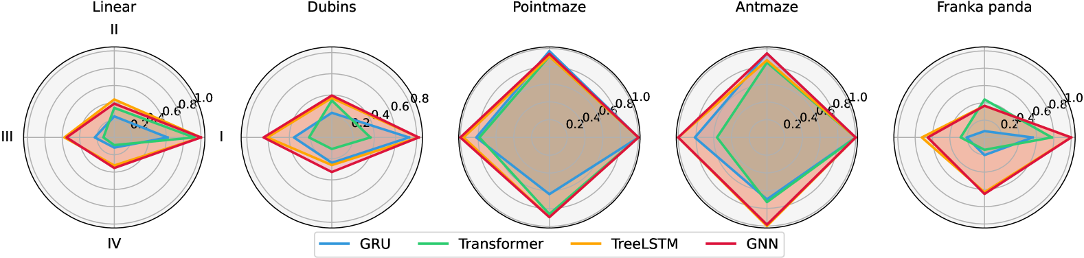
Figure 7: STL satisfaction rate distribution for different categories (I. single-goal; II. multi-goal; III. sequential; IV. partial).

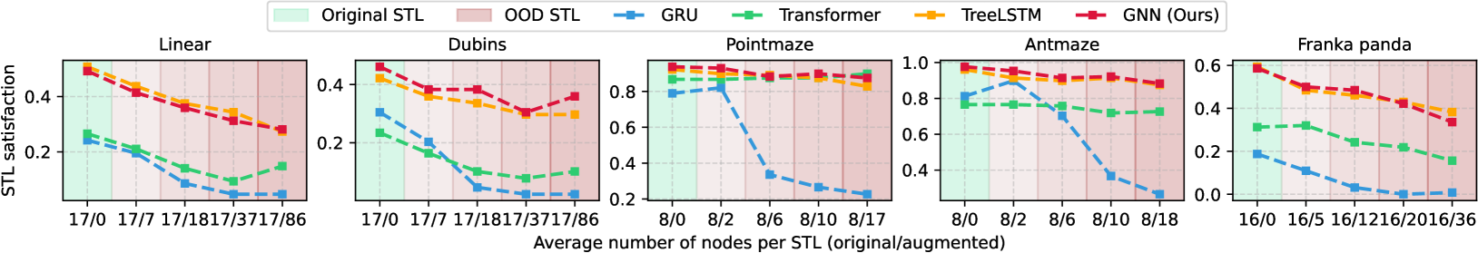
Figure 8: Encoder robustness test under varied STL augmentation (shaded in red). Graph-based encoders (GNN, TreeLSTM) demonstrate greater resilience to synthetic modifications compared to sequence-based models (GRU, Transformer).

5.3 Ablation study on encoder designs for STL

We compare different architectures to encode STL syntax, including sequence models like GRU and Transformer, and graph-encoding: GNN and TreeLSTM. We use the same pipeline as TeLoGraF, and only change the encoder network. As shown in Fig.5, all the encoders have a close to 100%percent 100 100%100 % satisfaction rate on the training splits, indicating they can distinguish different STL syntax. However, their abilities to generalize to unseen STL syntax are different: GRU and Transformer get lower STL scores than TreeLSTM and GNN; one reason could be that the graph-encoding models inherit permutation-invariance of the syntax tree (“A∨\lor∨B” is the same as “B∨\lor∨A”), making the learning more efficient. The performance of TreeLSTM and GNN are similar, and we select GNN encoding owing to its brevity.

5.4 Encoder coverage analysis on varied STL types

We show the validation STL satisfaction over different STL categories in Fig.7. As expected, most encoders can lead to high satisfaction rate on single-goal STLs. The improvements of the graph-encoding over sequence models are mainly from “Sequential” and “Partial” types, which implies that, beyond permutation-invariance, graph-encoding methods also excel at propagating time constraints and temporal orderings than the sequence models. However, all models’ performance on II-IV STLs is relatively low on Linear, Dubins and Franka Panda, which implies it is challenging for current models to generalize to complex STLs such as multi-goal satisfaction, sequential, or partial constraints. This highlights the value of our dataset in examining the limitation of the current models in handling complex STLs. Future improvements in architectures or training strategies are necessary to foster better temporal logic planning.

5.5 Robustness test for encoders on out-domain STLs

We alter the STLs in the validation splits and use the pre-trained models on the original dataset to produce trajectories. We deliberately keep the trajectories fixed and only change the STLs to ensure the backbone is not affected by out-of-distribution trajectories. For each ∧\land∧ and ∨\lor∨ operator in the STL syntax tree, we randomly duplicate a number of their children nodes (e.g., “A∧\land∧B” →→\to→ “A∧\land∧B∧\land∧B”). This augmentation will not affect the solutions. Ideally, if the model is robust, the output should have the same STL satisfaction rate. As shown in Fig.8, all models result in degradation as the number of nodes augmented increases, but the graph-based encoder (GNN, TreeLSTM) is resilient to the augmentation. In most out-domain cases, they can even outperform the sequence models with normal STL inputs. This implies graph-based encoders inherently capture the structural STL more effectively and generalize better under augmentations.

Limitations. First, TeLoGraF is data-driven and does not offer soundness and completeness guarantees as other classical planning methods. Its performance degrades for tasks with complex STL syntax or STL syntax that are heavily out-of-distribution. This limitation is inherent to most learning-based methods, as they rely on the distribution of training data. Trajectory refinement with classical methods could enhance the model’s generalization and robustness on these temporal logic tasks. We leave this for future work.

6 Conclusion

We propose TeLoGraF, a novel learning-based framework for solving general Signal Temporal Logic (STL) tasks via graph-encoding and flow-matching. TeLoGraF can handle flexible forms of specifications and outperforms existing classical and data-driven baselines while maintaining fast inference speed. Our analysis highlights the value of graph-based STL encoding. Aside from TeLoGraF, we introduce a new dataset for temporal logic planning, addressing the lack of diverse and structured STL benchmarks. Future research directions include improving the model’s generalization and robustness towards more complex temporal logic structure and out-of-distribution STL specifications.

Impact Statement

This paper presents work whose goal is to advance the field of robotics and decision-making for long-horizon tasks. There are some potential societal consequences of our work, for example, a fully-autonomous robot using our designed algorithm for decision-making could lead to potentially unsafe behavior. Thus, a safety-filter or backup policy for the planned behavior is needed for deployment. No other aspects which we feel must be specifically highlighted here.

References

• Carvalho et al. (2023) Carvalho, J., Le, A.T., Baierl, M., Koert, D., and Peters, J. Motion planning diffusion: Learning and planning of robot motions with diffusion models. In 2023 IEEE/RSJ International Conference on Intelligent Robots and Systems (IROS), pp. 1916–1923. IEEE, 2023.
• Chang et al. (2022) Chang, W.-D., Higuera, J. C.G., Fujimoto, S., Meger, D., and Dudek, G. Il-flow: Imitation learning from observation using normalizing flows. arXiv preprint arXiv:2205.09251, 2022.
• Chen et al. (2024) Chen, C., Deng, F., Kawaguchi, K., Gulcehre, C., and Ahn, S. Simple hierarchical planning with diffusion. arXiv preprint arXiv:2401.02644, 2024.
• Chen et al. (2023) Chen, Y., Li, H., and Zhao, D. Boosting continuous control with consistency policy. arXiv preprint arXiv:2310.06343, 2023.
• Chi et al. (2023) Chi, C., Xu, Z., Feng, S., Cousineau, E., Du, Y., Burchfiel, B., Tedrake, R., and Song, S. Diffusion policy: Visuomotor policy learning via action diffusion. The International Journal of Robotics Research, pp. 02783649241273668, 2023.
• Chung et al. (2014) Chung, J., Gulcehre, C., Cho, K., and Bengio, Y. Empirical evaluation of gated recurrent neural networks on sequence modeling. arXiv preprint arXiv:1412.3555, 2014.
• Clarke & Emerson (1981) Clarke, E.M. and Emerson, E.A. Design and synthesis of synchronization skeletons using branching time temporal logic. In Workshop on logic of programs, pp. 52–71. Springer, 1981.
• Coumans & Bai (2021) Coumans, E. and Bai, Y. Pybullet quickstart guide, 2021.
• Dawson & Fan (2022) Dawson, C. and Fan, C. Robust counterexample-guided optimization for planning from differentiable temporal logic. In 2022 IEEE/RSJ International Conference on Intelligent Robots and Systems (IROS), pp. 7205–7212. IEEE, 2022.
• de Lazcano et al. (2024) de Lazcano, R., Andreas, K., Tai, J.J., Lee, S.R., and Terry, J. Gymnasium robotics, 2024. URL http://github.com/Farama-Foundation/Gymnasium-Robotics.
• Donzé & Maler (2010) Donzé, A. and Maler, O. Robust satisfaction of temporal logic over real-valued signals. Formal Modeling and Analysis of Timed Systems, pp.92, 2010.
• Donzé et al. (2013) Donzé, A., Ferrere, T., and Maler, O. Efficient robust monitoring for stl. In Computer Aided Verification: 25th International Conference, CAV 2013, pp. 264–279. Springer, 2013.
• Eappen et al. (2025) Eappen, J., Xiong, Z., Patel, D., Bera, A., and Jagannathan, S. Scaling safe multi-agent control for signal temporal logic specifications. arXiv preprint arXiv:2501.05639, 2025.
• Fainekos et al. (2009) Fainekos, G.E., Girard, A., Kress-Gazit, H., and Pappas, G.J. Temporal logic motion planning for dynamic robots. Automatica, 45(2):343–352, 2009.
• Fang et al. (2024) Fang, X., Garrett, C.R., Eppner, C., Lozano-Pérez, T., Kaelbling, L.P., and Fox, D. Dimsam: Diffusion models as samplers for task and motion planning under partial observability. In 2024 IEEE/RSJ International Conference on Intelligent Robots and Systems (IROS), pp. 1412–1419. IEEE, 2024.
• Feng et al. (2024) Feng, Z., Luan, H., Goyal, P., and Soh, H. Ltldog: Satisfying temporally-extended symbolic constraints for safe diffusion-based planning. arXiv preprint arXiv:2405.04235, 2024.
• Fey & Lenssen (2019) Fey, M. and Lenssen, J.E. Fast graph representation learning with pytorch geometric. arXiv preprint arXiv:1903.02428, 2019.
• Finucane et al. (2010) Finucane, C., Jing, G., and Kress-Gazit, H. Ltlmop: Experimenting with language, temporal logic and robot control. In 2010 IEEE/RSJ International Conference on Intelligent Robots and Systems, pp. 1988–1993. IEEE, 2010.
• Fu et al. (2020) Fu, J., Kumar, A., Nachum, O., Tucker, G., and Levine, S. D4rl: Datasets for deep data-driven reinforcement learning. arXiv preprint arXiv:2004.07219, 2020.
• Gaz et al. (2019) Gaz, C., Cognetti, M., Oliva, A., Giordano, P.R., and De Luca, A. Dynamic identification of the franka emika panda robot with retrieval of feasible parameters using penalty-based optimization. IEEE Robotics and Automation Letters, 4(4):4147–4154, 2019.
• Guo et al. (2024) Guo, Z., Zhou, W., and Li, W. Temporal logic specification-conditioned decision transformer for offline safe reinforcement learning. In Forty-first International Conference on Machine Learning, 2024.
• Hashimoto et al. (2022) Hashimoto, W., Hashimoto, K., Kishida, M., and Takai, S. Neural controller synthesis for signal temporal logic specifications using encoder-decoder structured networks. arXiv preprint arXiv:2212.05200, 2022.
• He et al. (2022) He, J., Bartocci, E., Ničković, D., Isakovic, H., and Grosu, R. Deepstl: from english requirements to signal temporal logic. In Proceedings of the 44th International Conference on Software Engineering, pp. 610–622, 2022.
• Ho et al. (2020) Ho, J., Jain, A., and Abbeel, P. Denoising diffusion probabilistic models. Advances in neural information processing systems, 2020.
• Huang et al. (2024) Huang, H., Sundaralingam, B., Mousavian, A., Murali, A., Goldberg, K., and Fox, D. Diffusionseeder: Seeding motion optimization with diffusion for rapid motion planning. arXiv preprint arXiv:2410.16727, 2024.
• Jackermeier & Abate (2024) Jackermeier, M. and Abate, A. Deepltl: Learning to efficiently satisfy complex ltl specifications. arXiv preprint arXiv:2410.04631, 2024.
• Janner et al. (2022) Janner, M., Du, Y., Tenenbaum, J.B., and Levine, S. Planning with diffusion for flexible behavior synthesis. arXiv preprint arXiv:2205.09991, 2022.
• Kapoor et al. (2020) Kapoor, P., Balakrishnan, A., and Deshmukh, J.V. Model-based reinforcement learning from signal temporal logic specifications. arXiv preprint arXiv:2011.04950, 2020.
• Ke et al. (2024) Ke, T.-W., Gkanatsios, N., and Fragkiadaki, K. 3d diffuser actor: Policy diffusion with 3d scene representations. arXiv preprint arXiv:2402.10885, 2024.
• Kiefer (2020) Kiefer, S. Power and limits of the Weisfeiler-Leman algorithm. PhD thesis, Dissertation, RWTH Aachen University, 2020, 2020.
• Kingma (2014) Kingma, D. Adam: a method for stochastic optimization. arXiv preprint arXiv:1412.6980, 2014.
• Kipf & Welling (2016) Kipf, T.N. and Welling, M. Semi-supervised classification with graph convolutional networks. arXiv preprint arXiv:1609.02907, 2016.
• Koymans (1990) Koymans, R. Specifying real-time properties with metric temporal logic. Real-time systems, 2(4):255–299, 1990.
• Kurtz & Lin (2022) Kurtz, V. and Lin, H. Mixed-integer programming for signal temporal logic with fewer binary variables. IEEE Control Systems Letters, 6:2635–2640, 2022.
• Leung & Pavone (2022) Leung, K. and Pavone, M. Semi-supervised trajectory-feedback controller synthesis for signal temporal logic specifications. In 2022 American Control Conference (ACC), pp. 178–185. IEEE, 2022.
• Leung et al. (2023) Leung, K., Aréchiga, N., and Pavone, M. Backpropagation through signal temporal logic specifications: Infusing logical structure into gradient-based methods. The International Journal of Robotics Research, 42(6):356–370, 2023.
• Li et al. (2023) Li, W., Wang, X., Jin, B., and Zha, H. Hierarchical diffusion for offline decision making. In International Conference on Machine Learning, pp. 20035–20064. PMLR, 2023.
• Li et al. (2017) Li, X., Vasile, C.-I., and Belta, C. Reinforcement learning with temporal logic rewards. In 2017 IEEE/RSJ International Conference on Intelligent Robots and Systems (IROS), pp. 3834–3839. IEEE, 2017.
• Liu et al. (2021) Liu, W., Mehdipour, N., and Belta, C. Recurrent neural network controllers for signal temporal logic specifications subject to safety constraints. IEEE Control Systems Letters, 6:91–96, 2021.
• Liu et al. (2022) Liu, X., Gong, C., and Liu, Q. Flow straight and fast: Learning to generate and transfer data with rectified flow. arXiv preprint arXiv:2209.03003, 2022.
• Maierhofer et al. (2022) Maierhofer, S., Moosbrugger, P., and Althoff, M. Formalization of intersection traffic rules in temporal logic. In 2022 IEEE Intelligent Vehicles Symposium (IV), pp. 1135–1144. IEEE, 2022.
• Maler & Nickovic (2004) Maler, O. and Nickovic, D. Monitoring temporal properties of continuous signals. Formal Techniques, ModellingandAnalysis of Timed and Fault-Tolerant Systems, pp. 152, 2004.
• Meng & Fan (2023) Meng, Y. and Fan, C. Signal temporal logic neural predictive control. IEEE Robotics and Automation Letters, 2023.
• Meng & Fan (2024) Meng, Y. and Fan, C. Diverse controllable diffusion policy with signal temporal logic. IEEE Robotics and Automation Letters, 2024.
• Mishra et al. (2023) Mishra, U.A., Xue, S., Chen, Y., and Xu, D. Generative skill chaining: Long-horizon skill planning with diffusion models. In Conference on Robot Learning, pp. 2905–2925. PMLR, 2023.
• Nair & Hinton (2010) Nair, V. and Hinton, G.E. Rectified linear units improve restricted boltzmann machines. In Proceedings of the 27th international conference on machine learning (ICML-10), pp. 807–814, 2010.
• Paszke et al. (2019) Paszke, A., Gross, S., Massa, F., Lerer, A., Bradbury, J., Chanan, G., Killeen, T., Lin, Z., Gimelshein, N., Antiga, L., et al. Pytorch: An imperative style, high-performance deep learning library. Advances in neural information processing systems, 32, 2019.
• Pnueli (1977) Pnueli, A. The temporal logic of programs. In 18th annual symposium on foundations of computer science (sfcs 1977), pp. 46–57. ieee, 1977.
• Prasad et al. (2024) Prasad, A., Lin, K., Wu, J., Zhou, L., and Bohg, J. Consistency policy: Accelerated visuomotor policies via consistency distillation. arXiv preprint arXiv:2405.07503, 2024.
• Puranic et al. (2021) Puranic, A., Deshmukh, J., and Nikolaidis, S. Learning from demonstrations using signal temporal logic. In Conference on Robot Learning, pp. 2228–2242. PMLR, 2021.
• Raman et al. (2015) Raman, V., Donzé, A., Sadigh, D., Murray, R.M., and Seshia, S.A. Reactive synthesis from signal temporal logic specifications. In Proceedings of the 18th international conference on hybrid systems: Computation and control, pp. 239–248, 2015.
• Sadraddini & Belta (2015) Sadraddini, S. and Belta, C. Robust temporal logic model predictive control. In 2015 53rd Annual Allerton Conference on Communication, Control, and Computing (Allerton), pp. 772–779. IEEE, 2015.
• Sun et al. (2022) Sun, D., Chen, J., Mitra, S., and Fan, C. Multi-agent motion planning from signal temporal logic specifications. IEEE Robotics and Automation Letters, 7(2):3451–3458, 2022.
• Tai et al. (2015) Tai, K.S., Socher, R., and Manning, C.D. Improved semantic representations from tree-structured long short-term memory networks. arXiv preprint arXiv:1503.00075, 2015.
• Team et al. (2024) Team, O.M., Ghosh, D., Walke, H., Pertsch, K., Black, K., Mees, O., Dasari, S., Hejna, J., Kreiman, T., Xu, C., et al. Octo: An open-source generalist robot policy. arXiv preprint arXiv:2405.12213, 2024.
• Todorov et al. (2012) Todorov, E., Erez, T., and Tassa, Y. Mujoco: A physics engine for model-based control. In 2012 IEEE/RSJ international conference on intelligent robots and systems, pp. 5026–5033. IEEE, 2012.
• Urain et al. (2024) Urain, J., Mandlekar, A., Du, Y., Shafiullah, M., Xu, D., Fragkiadaki, K., Chalvatzaki, G., and Peters, J. Deep generative models in robotics: A survey on learning from multimodal demonstrations. arXiv preprint arXiv:2408.04380, 2024.
• Vasile et al. (2017) Vasile, C.-I., Raman, V., and Karaman, S. Sampling-based synthesis of maximally-satisfying controllers for temporal logic specifications. In 2017 IEEE/RSJ International Conference on Intelligent Robots and Systems (IROS), pp. 3840–3847. IEEE, 2017.
• Vaswani (2017) Vaswani, A. Attention is all you need. Advances in Neural Information Processing Systems, 2017.
• Wongpiromsarn et al. (2012) Wongpiromsarn, T., Topcu, U., and Murray, R.M. Receding horizon temporal logic planning. IEEE Transactions on Automatic Control, 57(11):2817–2830, 2012.
• Xian et al. (2023) Xian, Z., Gkanatsios, N., Gervet, T., Ke, T.-W., and Fragkiadaki, K. Chaineddiffuser: Unifying trajectory diffusion and keypose prediction for robotic manipulation. In 7th Annual Conference on Robot Learning, 2023.
• Xu et al. (2018) Xu, K., Hu, W., Leskovec, J., and Jegelka, S. How powerful are graph neural networks? arXiv preprint arXiv:1810.00826, 2018.
• Yang et al. (2023) Yang, Z., Mao, J., Du, Y., Wu, J., Tenenbaum, J.B., Lozano-Pérez, T., and Kaelbling, L.P. Compositional diffusion-based continuous constraint solvers. arXiv preprint arXiv:2309.00966, 2023.
• Ze et al. (2024) Ze, Y., Zhang, G., Zhang, K., Hu, C., Wang, M., and Xu, H. 3d diffusion policy. arXiv preprint arXiv:2403.03954, 2024.
• Zhang et al. (2024) Zhang, Q., Liu, Z., Fan, H., Liu, G., Zeng, B., and Liu, S. Flowpolicy: Enabling fast and robust 3d flow-based policy via consistency flow matching for robot manipulation. arXiv preprint arXiv:2412.04987, 2024.
• Zhong et al. (2024) Zhong, S., Power, T., Gupta, A., and Mitrano, P. PyTorch Kinematics, February 2024.
• Zhong et al. (2023) Zhong, Z., Rempe, D., Xu, D., Chen, Y., Veer, S., Che, T., Ray, B., and Pavone, M. Guided conditional diffusion for controllable traffic simulation. In 2023 IEEE International Conference on Robotics and Automation (ICRA), pp. 3560–3566. IEEE, 2023.

Appendix A Experiment setups

A.1 Simulation Environments

A.1.1 Linear

We use a single-integrator dynamic model. The 2D state (x,y)𝑥 𝑦(x,y)( italic_x , italic_y ) represents the 2D coordinates on a x⁢y 𝑥 𝑦 xy italic_x italic_y-plane, and the 2D control input (u,v)𝑢 𝑣(u,v)( italic_u , italic_v ) reflects the velocities in these two directions. We set the time step duration Δ⁢t=0.5 Δ 𝑡 0.5\Delta t=0.5 roman_Δ italic_t = 0.5. The system dynamic is described as:

{x t+1=x t+u t⁢Δ⁢t y t+1=y t+v t⁢Δ⁢t cases subscript 𝑥 𝑡 1 absent subscript 𝑥 𝑡 subscript 𝑢 𝑡 Δ 𝑡 subscript 𝑦 𝑡 1 absent subscript 𝑦 𝑡 subscript 𝑣 𝑡 Δ 𝑡\begin{cases}x_{t+1}&=x_{t}+u_{t}\Delta t\ y_{t+1}&=y_{t}+v_{t}\Delta t\ \end{cases}{ start_ROW start_CELL italic_x start_POSTSUBSCRIPT italic_t + 1 end_POSTSUBSCRIPT end_CELL start_CELL = italic_x start_POSTSUBSCRIPT italic_t end_POSTSUBSCRIPT + italic_u start_POSTSUBSCRIPT italic_t end_POSTSUBSCRIPT roman_Δ italic_t end_CELL end_ROW start_ROW start_CELL italic_y start_POSTSUBSCRIPT italic_t + 1 end_POSTSUBSCRIPT end_CELL start_CELL = italic_y start_POSTSUBSCRIPT italic_t end_POSTSUBSCRIPT + italic_v start_POSTSUBSCRIPT italic_t end_POSTSUBSCRIPT roman_Δ italic_t end_CELL end_ROW(6)

In this environment, we randomly generate goal regions and obstacles in a circle shape, and generate STL specifications using procedural methods. Finally, we use a gradient-based trajectory optimization method implemented in PyTorch(Paszke et al., 2019) to compute the demonstration trajectories. The loss function is constructed as:

ℒ=min⁡(0.5−ρ⁢(τ,0,ϕ),0)+c 1⁢1 T⁢∑t=0 T{min⁡(u t 2−1,0)+min⁡(v t 2−1,0)}+c 2⁢1 T⁢∑t=0 T(u t 2+v t 2)ℒ 0.5 𝜌 𝜏 0 italic-ϕ 0 subscript 𝑐 1 1 𝑇 superscript subscript 𝑡 0 𝑇 superscript subscript 𝑢 𝑡 2 1 0 superscript subscript 𝑣 𝑡 2 1 0 subscript 𝑐 2 1 𝑇 superscript subscript 𝑡 0 𝑇 superscript subscript 𝑢 𝑡 2 superscript subscript 𝑣 𝑡 2\mathcal{L}=\min(0.5-\rho(\tau,0,\phi),0)+c_{1}\frac{1}{T}\sum\limits_{t=0}^{T% }{\min(u_{t}^{2}-1,0)+\min(v_{t}^{2}-1,0)}+c_{2}\frac{1}{T}\sum\limits_{t=0}% ^{T}\limits(u_{t}^{2}+v_{t}^{2})caligraphic_L = roman_min ( 0.5 - italic_ρ ( italic_τ , 0 , italic_ϕ ) , 0 ) + italic_c start_POSTSUBSCRIPT 1 end_POSTSUBSCRIPT divide start_ARG 1 end_ARG start_ARG italic_T end_ARG ∑ start_POSTSUBSCRIPT italic_t = 0 end_POSTSUBSCRIPT start_POSTSUPERSCRIPT italic_T end_POSTSUPERSCRIPT { roman_min ( italic_u start_POSTSUBSCRIPT italic_t end_POSTSUBSCRIPT start_POSTSUPERSCRIPT 2 end_POSTSUPERSCRIPT - 1 , 0 ) + roman_min ( italic_v start_POSTSUBSCRIPT italic_t end_POSTSUBSCRIPT start_POSTSUPERSCRIPT 2 end_POSTSUPERSCRIPT - 1 , 0 ) } + italic_c start_POSTSUBSCRIPT 2 end_POSTSUBSCRIPT divide start_ARG 1 end_ARG start_ARG italic_T end_ARG ∑ start_POSTSUBSCRIPT italic_t = 0 end_POSTSUBSCRIPT start_POSTSUPERSCRIPT italic_T end_POSTSUPERSCRIPT ( italic_u start_POSTSUBSCRIPT italic_t end_POSTSUBSCRIPT start_POSTSUPERSCRIPT 2 end_POSTSUPERSCRIPT + italic_v start_POSTSUBSCRIPT italic_t end_POSTSUBSCRIPT start_POSTSUPERSCRIPT 2 end_POSTSUPERSCRIPT )(7)

The first loss term maximizes the truncated robustness score ρ 𝜌\rho italic_ρ for the trajectory τ=(x 0,u 0,…,u T−1,x T)𝜏 subscript 𝑥 0 subscript 𝑢 0…subscript 𝑢 𝑇 1 subscript 𝑥 𝑇\tau=(x_{0},u_{0},...,u_{T-1},x_{T})italic_τ = ( italic_x start_POSTSUBSCRIPT 0 end_POSTSUBSCRIPT , italic_u start_POSTSUBSCRIPT 0 end_POSTSUBSCRIPT , … , italic_u start_POSTSUBSCRIPT italic_T - 1 end_POSTSUBSCRIPT , italic_x start_POSTSUBSCRIPT italic_T end_POSTSUBSCRIPT ) to ensure STL rule satisfaction for the STL ϕ italic-ϕ\phi italic_ϕ. The second loss term regulates the magnitude of the control input to be within 1. The third loss term minimizes the control magnitude to make the trajectory smooth.

A.1.2 Dubins

We use a car-like dynamic model. The 4D state (x,y,θ,v)𝑥 𝑦 𝜃 𝑣(x,y,\theta,v)( italic_x , italic_y , italic_θ , italic_v ) represents the 2D coordinates on the x⁢y 𝑥 𝑦 xy italic_x italic_y-plane, the heading angle of the robot and the velocity of the robot, respectively. The 2D control input (ω,a)𝜔 𝑎(\omega,a)( italic_ω , italic_a ) represents the angular velocity and the acceleration. We set the time step duration Δ⁢t=0.5 Δ 𝑡 0.5\Delta t=0.5 roman_Δ italic_t = 0.5. The system dynamic is described as:

{x t+1=x t+v t⁢cos⁡(θ t)⁢Δ⁢t y t+1=y t+v t⁢sin⁡(θ t)⁢Δ⁢t θ t+1=θ t+ω t⁢Δ⁢t v t+1=v t+a t⁢Δ⁢t cases subscript 𝑥 𝑡 1 absent subscript 𝑥 𝑡 subscript 𝑣 𝑡 subscript 𝜃 𝑡 Δ 𝑡 subscript 𝑦 𝑡 1 absent subscript 𝑦 𝑡 subscript 𝑣 𝑡 subscript 𝜃 𝑡 Δ 𝑡 subscript 𝜃 𝑡 1 absent subscript 𝜃 𝑡 subscript 𝜔 𝑡 Δ 𝑡 subscript 𝑣 𝑡 1 absent subscript 𝑣 𝑡 subscript 𝑎 𝑡 Δ 𝑡\begin{cases}x_{t+1}&=x_{t}+v_{t}\cos(\theta_{t})\Delta t\ y_{t+1}&=y_{t}+v_{t}\sin(\theta_{t})\Delta t\ \theta_{t+1}&=\theta_{t}+\omega_{t}\Delta t\ v_{t+1}&=v_{t}+a_{t}\Delta t\ \end{cases}{ start_ROW start_CELL italic_x start_POSTSUBSCRIPT italic_t + 1 end_POSTSUBSCRIPT end_CELL start_CELL = italic_x start_POSTSUBSCRIPT italic_t end_POSTSUBSCRIPT + italic_v start_POSTSUBSCRIPT italic_t end_POSTSUBSCRIPT roman_cos ( italic_θ start_POSTSUBSCRIPT italic_t end_POSTSUBSCRIPT ) roman_Δ italic_t end_CELL end_ROW start_ROW start_CELL italic_y start_POSTSUBSCRIPT italic_t + 1 end_POSTSUBSCRIPT end_CELL start_CELL = italic_y start_POSTSUBSCRIPT italic_t end_POSTSUBSCRIPT + italic_v start_POSTSUBSCRIPT italic_t end_POSTSUBSCRIPT roman_sin ( italic_θ start_POSTSUBSCRIPT italic_t end_POSTSUBSCRIPT ) roman_Δ italic_t end_CELL end_ROW start_ROW start_CELL italic_θ start_POSTSUBSCRIPT italic_t + 1 end_POSTSUBSCRIPT end_CELL start_CELL = italic_θ start_POSTSUBSCRIPT italic_t end_POSTSUBSCRIPT + italic_ω start_POSTSUBSCRIPT italic_t end_POSTSUBSCRIPT roman_Δ italic_t end_CELL end_ROW start_ROW start_CELL italic_v start_POSTSUBSCRIPT italic_t + 1 end_POSTSUBSCRIPT end_CELL start_CELL = italic_v start_POSTSUBSCRIPT italic_t end_POSTSUBSCRIPT + italic_a start_POSTSUBSCRIPT italic_t end_POSTSUBSCRIPT roman_Δ italic_t end_CELL end_ROW(8)

In this environment, we randomly generate goal regions and obstacles in a circle shape, and generate STL specifications using procedural methods. Finally, we use a gradient-based trajectory optimization method implemented in PyTorch(Paszke et al., 2019) to compute the demonstration trajectories. The loss is similar to Eq.(8).

A.1.3 PointMaze

We adapt PointMaze and AntMaze from these two environments from(Fu et al., 2020). The original environments consist of 2D navigation tasks where an agent must navigate a maze to reach a goal while avoiding obstacles. The dynamic model is internally handled by MuJoCo(Todorov et al., 2012), and we use the Gymnasium-Robotics package(de Lazcano et al., 2024) for simulation to collect data. We use the largest maze in both simulations with horizons set as 512 steps. In Pointmaze, the agent is modeled as a simple 2D point mass with position (x,y)𝑥 𝑦(x,y)( italic_x , italic_y ) and the control input is the linear force along xy directions. We collect the 4-dimension trajectory with 2d xy-coordinate and 2d control input. To collect trajectories, we first generate the skeleton of the STL syntax but leave the time intervals as placeholders; then, we use a planning algorithm to find waypoints and then use a PD goal-reaching controller to collect trajectories. After the generation of the trajectories, we first ensure it reaches the final destination, and then we evaluate the robustness score on the trajectory without considering the time intervals. If the robustness score is positive, we randomly infer the possible time intervals for the goal-reaching sub-formulas and run post-verification to ensure the trajectory satisfies this STL.

A.1.4 AntMaze

In AntMaze, the agent is modeled as a more complex 8-DoF quadruped robot with 27-dimension observation (1-dimension for z-coordinate of the torso, 4-dimension for the torso orientation (in Quaternion representation), 3-dimension velocity and 3-dimension angular velocity for the torso, 8-dimension for each of the joints’ angles and another 8-dimension for each of the joints’ angular velocities), 8-dimension control input serving as the torques applied to each of the 8 joint rotors, and an extra 2-dimension for the xy-coordinates of the torso. We collect the 10-dimension trajectory with 2d xy-coordinate and 8-dimension control input. We adopt similar data collection methods as in PointMaze, with the difference of switching from PD controller to a RL goal-reaching policy.

A.1.5 Franka Panda

We use a 7 DoF Franka Panda robot arm model and conduct the simulation via PyBullet Simulator(Coumans & Bai, 2021). We use the standard URDF files to construct the scene: a table is generated via “table.urdf” at location [0.4,0,0]0.4 0 0[0.4,0,0][ 0.4 , 0 , 0 ] with Euler angle [0,0,n⁢p.p⁢i/2]delimited-[]formulae-sequence 0 0 𝑛 𝑝 𝑝 𝑖 2[0,0,np.pi/2][ 0 , 0 , italic_n italic_p . italic_p italic_i / 2 ]. A Franka Panda robot is generated via “franka/panda.urdf” at location [0,0,0.6]0 0 0.6[0,0,0.6][ 0 , 0 , 0.6 ] with Euler angle [0,0,0]0 0 0[0,0,0][ 0 , 0 , 0 ]. The 7DoF joint angles for the robot are initialized at (in radian) [0.0000,0.0000,0.0000,−2.0000,0.0000,1.8675,0.0000]0.0000 0.0000 0.0000 2.0000 0.0000 1.8675 0.0000[0.0000,0.0000,0.0000,-2.0000,0.0000,1.8675,0.0000][ 0.0000 , 0.0000 , 0.0000 , - 2.0000 , 0.0000 , 1.8675 , 0.0000 ] and are clipped from [−2.8972,−1.7628,−2.8972,−3.0718,−2.8972,−0.0175,−2.8972]2.8972 1.7628 2.8972 3.0718 2.8972 0.0175 2.8972[-2.8972,-1.7628,-2.8972,-3.0718,-2.8972,-0.0175,-2.8972][ - 2.8972 , - 1.7628 , - 2.8972 , - 3.0718 , - 2.8972 , - 0.0175 , - 2.8972 ] to [2.8972,1.7628,2.8972,−0.0698,2.8972,3.7525,2.8972]2.8972 1.7628 2.8972 0.0698 2.8972 3.7525 2.8972[2.8972,1.7628,2.8972,-0.0698,2.8972,3.7525,2.8972][ 2.8972 , 1.7628 , 2.8972 , - 0.0698 , 2.8972 , 3.7525 , 2.8972 ] by following the guidelines. Random goal objects are generated on the table whereas the obstacles are generated both on the table and in the midair to increase the task difficulty. We use a gradient-based method to plan the trajectory to satisfy the STL conditions. We use pytorch-kinematics(Zhong et al., 2024) library to leverage Pytorch and GPU devices to compute the forward kinematic in a parallelized and efficient way. The time horizon is 64 with the time step duration Δ⁢t=0.05 Δ 𝑡 0.05\Delta t=0.05 roman_Δ italic_t = 0.05.

A.2 Procedural methods to generate STL formulas

We adopt procedural methods to generate the STL formulas. We first assign the type of STL we want to generate (Single-goal, multi-goal, sequential, partial-order). Then each formula is augmented with randomly chosen 0-6 obstacles and 0-4 goals while they are not colliding with each other. Next, we spawn the agent position in the free space and use either search-planning-then-tracking method or end-to-end gradient-based method to collect the trajectories. More details are in the code, and here in the following section we will show a subset of demonstrations with the visualized STL syntax trees.

A.3 Baselines

A.3.1 Grad/Grad-lite

We directly use the data collection method we have for the three benchmarks, Linear, Dubins, and Panda. We set different gradient-descent iterations for the different environments. For Linear and Dubins, we set niters=10 for “Grad-lite” and niters=50 for “Grad”, and for Franka Panda environment, we set niters=50 for “Grad-lite” and niters=150 for “Grad”.

A.3.2 CEM

We use the Cross Entropy Method with the elite size of 25, the population sample size of 64, and the number of iteration steps is set to 100.

A.3.3 CTG

We followed the guidance in Zhong et al. (2023) and implemented this baseline by ourselves, as the original baseline is conducted for the autonomous driving dataset. To ensure we don’t have STL-condition-input encountered in training and to make a fair comparison with TeLoGraF backbone, we train a goal-conditioned flow-matching policy where the goal condition is constructed as a set of subgoals and obstacles (we also mark whether they are goals or obstacles in this embedding). At the inference stage, we use the gradient-based method to construct the guidance for the flow-matching model.

A.3.4 LTLDoG

Similar to CTG, we first train a goal-conditioned flow-matching policy. Further, we train an STL classifier as suggested in Feng et al. (2024). At each iteration, in the minibatch data we add noise to the demonstration data and compute their robustness score (they are most likely to be negative scores) for the corresponding STL. We also save the STL score for the existing demonstration trajectories. We train our STL classifier to predict the scores for both the original trajectories and the perturbed trajectories using a simple L2 loss (suggested in Feng et al. (2024)). With 50 epochs of training, on most benchmarks the STL classifier can already achieve more than 90%percent 90 90%90 % accuracy in classifying positive and negative sample trajectories regarding the STL specification (and since we need to evaluate the robustness score during training, the training is 10-20X slower than the flow-matching model training). We then use this trained STL classifier in the flow-matching generation process as guidance.

Appendix B Additional visualizations from our flow-matching model

Here we show the TeLoGraF generated trajectories on the Dubins benchmark and show how the trajectory distribution and satisfaction results change as the number of ODE steps decrease from 100 (the original setup for TeLoGraF) to 1. We plot the goals in blue color, obstacles in gray color, the initial state is plotted in a marker shape. The green trajectories are the demonstration data, and the red ones are the flow-model generated trajectories (we only plot 4 of them on each plot), where the dark red one is the generated trajectory with the highest robustness score for this STL. We can see that as the number of ODE steps decreases, the trajectories set become more ”concentrated”. The predicted trajectory can always satisfy the STL, until the last one (ODE steps=1) where the trajectory fails to reach goal-1, leading to a failure case.

(a)

(b)

Figure 9: Varied ODE steps, Dubins environment, TeLoGraF

(a)

(b)

Figure 10: Varied ODE steps, Dubins environment, TeLoGraF

(a)

(b)

Figure 11: Varied ODE steps, Dubins environment, TeLoGraF

(a)

(b)

Figure 12: Varied ODE steps, Dubins environment, TeLoGraF

Appendix C Additional visualizations from demonstration dataset

The results shown here are in the raw version (without data cleaning or improved visibility). Based on these data, we randomly select 2 demonstrations per STL listed in the dataset and collect 40K STLs for each of the benchmarks, gathering in total 200K STLs with 400K trajectories.

C.1 Linear environment

Here in the Linear environment, for one given STL, we actually start from eight different initial locations and initialize with 8 random control sequences for each initial location. The results satisfying the STL conditions (green) will be saved and the red ones are filtered out.

Figure 13: Linear environment. Single-goal STL

Figure 14: Linear environment. Single-goal STL

Figure 15: Linear environment. Multi-goal STL

Figure 16: Linear environment. Multi-goal STL

Figure 17: Linear environment. Sequential STL

Figure 18: Linear environment. Sequential STL

Figure 19: Linear environment. Partial STL

Figure 20: Linear environment. Partial STL

C.2 Dubins environment

In Dubin’s environment, the collected demonstration trajectories are more diverse and drastically change over time, owing to the large angular velocity and the acceleration rate.

Figure 21: Dubins environment. Single-goal STL

Figure 22: Dubins environment. Single-goal STL

Figure 23: Dubins environment. Multi-goal STL

Figure 24: Dubins environment. Multi-goal STL

Figure 25: Dubins environment. Sequential STL

Figure 26: Dubins environment. Sequential STL

Figure 27: Dubins environment. Partial STL

Figure 28: Dubins environment. Partial STL

C.3 PointMaze

Here, the pink trajectories are the demonstration data collected.

Figure 29: PointMaze environment. Single-goal STL

Figure 30: PointMaze environment. Multi-goal STL

Figure 31: PointMaze environment. Multi-goal STL

Figure 32: PointMaze environment. Sequential STL

Figure 33: PointMaze environment. Sequential STL

Figure 34: PointMaze environment. Sequential STL

Figure 35: PointMaze environment. Sequential STL

Figure 36: PointMaze environment. Partial STL

Figure 37: PointMaze environment. Partial STL

C.4 AntMaze

Here, the pink trajectories are the demonstration data collected.

Figure 38: AntMaze environment. Single-goal STL

Figure 39: AntMaze environment. Single-goal STL

Figure 40: AntMaze environment. Multi-goal STL

Figure 41: AntMaze environment. Multi-goal STL

Figure 42: AntMaze environment. Sequential STL

Figure 43: AntMaze environment. Sequential STL

Figure 44: AntMaze environment. Partial STL

Figure 45: AntMaze environment. Partial STL

C.5 Franka panda environment

Here, the blue trajectories in the last subfigure are the demonstrations that were collected.

Figure 46: Franka Panda environment. Single-goal STL

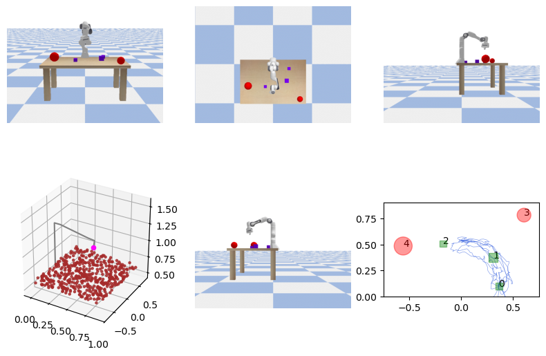
Figure 47: Franka Panda environment. Multi-goal STL

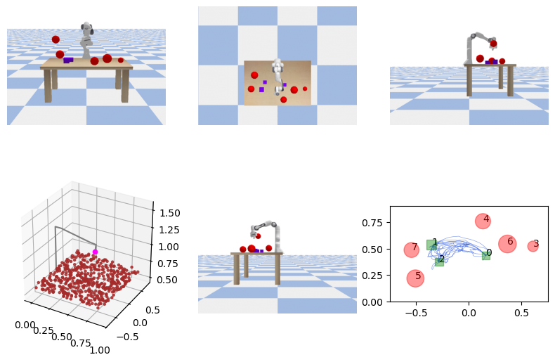
Figure 48: Franka Panda environment. Sequential STL

Figure 49: Franka Panda environment. Partial STL