2508/2508.00609.md

Title: Low-dimensional observer design for stable linear systems by model reduction

URL Source: https://arxiv.org/html/2508.00609

Published Time: Mon, 04 Aug 2025 00:38:38 GMT

Markdown Content: M.F. Shakib 1, M. Khalil 2,3, and R. Postoyan 2 1 Department of Electrical and Electronic Engineering, Imperial College London, London, UK (m.shakib@imperial.ac.uk).2 Université de Lorraine, CNRS, CRAN, F-54000 Nancy, France (firstname.surname@univ-lorraine.fr).3 Université de Lorraine, GREEN, F-54000 Nancy, France.This work has been partially supported by the Engineering and Physical Sciences Research Council, Grant EP/X033546/1.

Abstract

This paper presents a low-dimensional observer design for stable, single-input single-output, continuous-time linear time-invariant (LTI) systems. Leveraging the model reduction by moment matching technique, we approximate the system with a reduced-order model. Based on this reduced-order model, we design a low-dimensional observer that estimates the states of the original system. We show that this observer establishes exact asymptotic state reconstruction for a given class of inputs tied to the observer’s dimension. Furthermore, we establish an exponential input-to-state stability property for generic inputs, ensuring a bounded estimation error. Numerical simulations confirm the effectiveness of the approach for a benchmark model reduction problem.

I Introduction

In many applications, it is crucial to know the state of the dynamical system at hand, e.g., for state feedback or monitoring purposes. However, very often only the system output is measured rather than the full state. An observer-based approach may then be envisioned to estimate the state from input-output data. Such an observer takes the form of an auxiliary dynamical system, whose dimension is typically equal to or larger than the system dimension [1].

When the state dimension of the system is excessively large, designing as well as implementing an observer in real-time on devices with limited resources might be challenging or even infeasible. This challenge may arise when the plant model is obtained by spatially discretizing partial differential equations, like in, e.g., [2, 3, 4], or when considering networked systems, like in [5], for instance. A common technique to obtain an observer to reconstruct the full state of the system with a dimension smaller than that of the plant model is to proceed with a so-called reduced-order observer[6, 7, 8]. Reduced-order observers only estimate the state that cannot be directly inferred from measurements. By doing so, the observer dimension is reduced by the number of measured outputs, which is typically small. A different approach is proposed in [9], where it is explained how model reduction techniques can be exploited to derive a low-dimensional observer with guaranteed performance from a given Luenberger observer for an LTI plant model. When the plant exhibits a network structure, an alternative approach consists in designing a distributed observer, see, e.g., [10, 11], or an average state observer [12]. Ad-hoc solutions are also available for specific applications, like in, e.g., [5, 13] when dealing with battery packs. Despite these achievements, we generally lack methodological tools to design low-dimensional observers, which are able to generate estimates of the full state vector.

In this context, the problem considered in this article is to design an observer that reconstructs the full state of a (possibly large-scale) stable single-input single-output linear time-invariant (LTI) system, where the dimension of the observer dynamics is freely selected by the user as explained next. The main originality is to exploit recent advances in model order reduction [14] for this purpose. The approach that we envision is, in the first step, to approximate the dynamics of the system by a reduced-order model. Specifically, we use the interconnection-based moment matching technique[14]. A distinctive feature of this technique is that it provides a match between the steady-state response of the original plant and the steady-state response of the reduced-order model for user-defined classes of inputs characterized by so-called interpolation points. The dimension of the reduced-order model then directly relates to the number of interpolation points and, thereby, to the considered class of inputs. In the second step, we design an observer for the reduced-order model that has the same state dimension as the reduced-order model. The observer dimension is thus directly related to the user-defined class of inputs considered when performing the model order reduction. Finally, in the third step, we map the reconstructed state of the reduced-order model back to the non-reduced state of the original system. By doing so, we obtain an observer, which is able to reconstruct the full state of the original plant model, while typically having a much lower dimension. Moreover, the observer design only involves the matrices of the reduced model thereby facilitating its use as well as its implementation. Figure1 provides a schematic overview of the proposed approach.

Figure 1: Schematic overview of the proposed observer scheme with the system state dimension n n italic_n and the observer state dimension ν\nu italic_ν, typically smaller than n n italic_n. The observer is designed based on a reduced-order model of dimension ν\nu italic_ν.

We establish that the estimation error, i.e., the mismatch between the plant’s full state and its estimate generated by the low-dimensional observer, satisfies a global exponential input-to-state stability property. The “disturbance” term in this stability property corresponds to the mismatch between the actual system input and the closest input signal belonging to the class considered in the model reduction step through the choice of the interpolation points. Particularly, for inputs corresponding to these interpolation points, we show that this “disturbance term” is zero, and thus the estimation error tends to zero exponentially since the moment matching model reduction technique is exact for these inputs. This is despite a possibly, significantly smaller state dimension of the implemented observer, compared to the state dimension of the original system. In contrast to [9], we perform the model reduction directly on the plant rather than on a previously designed observer for the original system. This simplifies the design process, as we rely solely on the reduced-order model to synthesize the low-dimensional observer. Furthermore, exact asymptotic estimation is guaranteed whenever the input applied to the plant belongs to the class of inputs used for model reduction.

As mentioned above, we concentrate on stable single-input single-output linear time-invariant systems as a first step towards the exploitation of model order reduction techniques for observer design. As follow-up studies, we envision extending the proposed approach to different system classes such as, for example, unstable and nonlinear systems.

The remainder of this paper is organized as follows. Section II introduces the considered problem. Section III provides the background material on model reduction that is exploited in this work to design low-dimensional observers. Section IV presents the main theoretical contributions. Section V provides numerical examples showcasing the performance of the proposed method on a high-dimensional system. Section VI concludes the paper with a discussion of key findings and potential future directions.

Notation: Let ℝ\mathbb{R}blackboard_R, ℝ≥0\mathbb{R}{\geq 0}blackboard_R start_POSTSUBSCRIPT ≥ 0 end_POSTSUBSCRIPT, and ℝ>0\mathbb{R}{>0}blackboard_R start_POSTSUBSCRIPT > 0 end_POSTSUBSCRIPT denote the set of real, non-negative real, and positive real numbers, respectively. Let ℕ\mathbb{N}blackboard_N and ℕ>0\mathbb{N}{>0}blackboard_N start_POSTSUBSCRIPT > 0 end_POSTSUBSCRIPT be the set of non-negative and positive integers, respectively. We use ℂ\mathbb{C}blackboard_C, ℂ 0,ℂ−\mathbb{C}^{0},\mathbb{C}^{-}blackboard_C start_POSTSUPERSCRIPT 0 end_POSTSUPERSCRIPT , blackboard_C start_POSTSUPERSCRIPT - end_POSTSUPERSCRIPT, and ℂ+\mathbb{C}^{+}blackboard_C start_POSTSUPERSCRIPT + end_POSTSUPERSCRIPT to denote the set of complex numbers, and the set of complex numbers with zero real part, with negative real part and with positive real part, respectively. Given n∈ℕ>0 n\in\mathbb{N}{>0}italic_n ∈ blackboard_N start_POSTSUBSCRIPT > 0 end_POSTSUBSCRIPT, ℒ∞,n\mathcal{L}{\infty,n}caligraphic_L start_POSTSUBSCRIPT ∞ , italic_n end_POSTSUBSCRIPT stands for the set of functions from ℝ≥0\mathbb{R}{\geq 0}blackboard_R start_POSTSUBSCRIPT ≥ 0 end_POSTSUBSCRIPT to ℝ n\mathbb{R}^{n}blackboard_R start_POSTSUPERSCRIPT italic_n end_POSTSUPERSCRIPT that are locally essentially bounded and measurable, and we omit the index n n italic_n when the dimension is clear from the context. Given f∈ℒ∞f\in\mathcal{L}{\infty}italic_f ∈ caligraphic_L start_POSTSUBSCRIPT ∞ end_POSTSUBSCRIPT and t∈ℝ≥0 t\in\mathbb{R}{\geq 0}italic_t ∈ blackboard_R start_POSTSUBSCRIPT ≥ 0 end_POSTSUBSCRIPT, ‖f‖t|f|{t}∥ italic_f ∥ start_POSTSUBSCRIPT italic_t end_POSTSUBSCRIPT stands for ess​sup t′∈[0,t]‖f​(t′)‖\text{ess,}\sup{t^{\prime}\in[0,t]}|f(t^{\prime})|ess roman_sup start_POSTSUBSCRIPT italic_t start_POSTSUPERSCRIPT ′ end_POSTSUPERSCRIPT ∈ [ 0 , italic_t ] end_POSTSUBSCRIPT ∥ italic_f ( italic_t start_POSTSUPERSCRIPT ′ end_POSTSUPERSCRIPT ) ∥ where ∥⋅∥|\cdot|∥ ⋅ ∥ stands for the Euclidean norm. We use the notation ⟨⋅,⋅⟩\langle\cdot,\cdot\rangle⟨ ⋅ , ⋅ ⟩ for the scalar product of the considered Euclidean space, and ∇\nabla∇ for the nabla operator. Given a real, symmetric matrix P P italic_P, its largest and smallest eigenvalues are denoted by λ max​(P)\lambda_{\text{max}}(P)italic_λ start_POSTSUBSCRIPT max end_POSTSUBSCRIPT ( italic_P ) and λ min​(P)\lambda_{\text{min}}(P)italic_λ start_POSTSUBSCRIPT min end_POSTSUBSCRIPT ( italic_P ), respectively. We write rank(A)(A)( italic_A ) to denote the rank of a real matrix A A italic_A. Given a square real matrix A A italic_A, σ​(A)\sigma(A)italic_σ ( italic_A ) is the spectrum of A A italic_A and A≻0 A\succ 0 italic_A ≻ 0 means that A A italic_A is symmetric, positive definite. Furthermore, blockdiag​(A 1,A 2)\text{blockdiag}(A_{1},A_{2})blockdiag ( italic_A start_POSTSUBSCRIPT 1 end_POSTSUBSCRIPT , italic_A start_POSTSUBSCRIPT 2 end_POSTSUBSCRIPT ) denotes a block-diagonal matrix of square submatrices A 1 A_{1}italic_A start_POSTSUBSCRIPT 1 end_POSTSUBSCRIPT and A 2 A_{2}italic_A start_POSTSUBSCRIPT 2 end_POSTSUBSCRIPT. We write ‖A‖||A||| | italic_A | | to denote the 2 2 2-induced norm of the real square matrix A A italic_A. The imaginary unit −1\sqrt{-1}square-root start_ARG - 1 end_ARG is denoted by j j italic_j.

II Problem statement

We consider single-input single-output LTI systems described by the next state space representation

x˙=A​x+B​u,y=C​x,\dot{x}=Ax+Bu,\quad y=Cx,over˙ start_ARG italic_x end_ARG = italic_A italic_x + italic_B italic_u , italic_y = italic_C italic_x ,(1)

where, at time t∈ℝ≥0 t\in\mathbb{R}{\geq 0}italic_t ∈ blackboard_R start_POSTSUBSCRIPT ≥ 0 end_POSTSUBSCRIPT, x​(t)∈ℝ n x(t)\in\mathbb{R}^{n}italic_x ( italic_t ) ∈ blackboard_R start_POSTSUPERSCRIPT italic_n end_POSTSUPERSCRIPT is the state vector with n∈ℕ>0 n\in\mathbb{N}{>0}italic_n ∈ blackboard_N start_POSTSUBSCRIPT > 0 end_POSTSUBSCRIPT, u​(t)∈ℝ u(t)\in\mathbb{R}italic_u ( italic_t ) ∈ blackboard_R is the input, and y​(t)∈ℝ y(t)\in\mathbb{R}italic_y ( italic_t ) ∈ blackboard_R is the output. The matrices A,B,and​C A,B,\text{ and }C italic_A , italic_B , and italic_C are real-valued and have appropriate dimensions. We assume that the signal corresponding to u u italic_u belongs to ℒ∞\mathcal{L}_{\infty}caligraphic_L start_POSTSUBSCRIPT ∞ end_POSTSUBSCRIPT.

In many applications, the state x x italic_x of the system has to be known, while only the output y y italic_y of the system can be measured. In such a case, an observer, for example, a Luenberger observer, can be designed to reconstruct the unknown state when the pair (A,C)(A,C)( italic_A , italic_C ) is detectable. In particular, for system(1), such a Luenberger observer takes the form

x^˙=A​x^+B​u+M​(y−y^),y^=C​x^,\displaystyle\dot{\hat{x}}=A\hat{x}+Bu+M(y-\hat{y}),\quad\hat{y}=C\hat{x},over˙ start_ARG over^ start_ARG italic_x end_ARG end_ARG = italic_A over^ start_ARG italic_x end_ARG + italic_B italic_u + italic_M ( italic_y - over^ start_ARG italic_y end_ARG ) , over^ start_ARG italic_y end_ARG = italic_C over^ start_ARG italic_x end_ARG ,(2)

where, at time t∈ℝ≥0 t\in\mathbb{R}_{\geq 0}italic_t ∈ blackboard_R start_POSTSUBSCRIPT ≥ 0 end_POSTSUBSCRIPT, x^​(t)∈ℝ n\hat{x}(t)\in\mathbb{R}^{n}over^ start_ARG italic_x end_ARG ( italic_t ) ∈ blackboard_R start_POSTSUPERSCRIPT italic_n end_POSTSUPERSCRIPT is the estimated state vector, y^​(t)∈ℝ\hat{y}(t)\in\mathbb{R}over^ start_ARG italic_y end_ARG ( italic_t ) ∈ blackboard_R is the estimated output, and M∈ℝ n M\in\mathbb{R}^{n}italic_M ∈ blackboard_R start_POSTSUPERSCRIPT italic_n end_POSTSUPERSCRIPT is the observer gain. Assuming (A,C)(A,C)( italic_A , italic_C ) is detectable, a gain M M italic_M can always be designed such that A−M​C A-MC italic_A - italic_M italic_C is Hurwitz, i.e., σ​(A−M​C)⊂ℂ−\sigma(A-MC)\subset\mathbb{C}^{-}italic_σ ( italic_A - italic_M italic_C ) ⊂ blackboard_C start_POSTSUPERSCRIPT - end_POSTSUPERSCRIPT, which results in the global exponential convergence of the error e:=x−x^e:=x-\hat{x}italic_e := italic_x - over^ start_ARG italic_x end_ARG to zero along the solutions to (1), (2), see [15].

As evident from observer(2), the dimension of x^\hat{x}over^ start_ARG italic_x end_ARG is n n italic_n, which is equal to the state dimension of the original system(1). For large-scale systems, this presents a substantial challenge not just in designing the observer gain M M italic_M, but also in implementing the observer in real-time on devices with limited resources. The objective of this work is to provide a method to design a state-observer for system (1), whose dimension can be freely tuned by the user depending on the considered class of signals to which u u italic_u belongs to. Moreover, this observer has to generate estimates of the original full state vector x x italic_x, and not only of the unmeasured states as in reduced-order observers. We propose to leverage the model order reduction techniques in [14] for this purpose. The next section reviews relevant background. Throughout this article, we pose the following standing assumption.

Standing Assumption 1 (SA1)

System(1) is minimal and the matrix A A italic_A in(1) is Hurwitz, i.e., σ​(A)⊂ℂ−\sigma(A)\subset\mathbb{C}^{-}italic_σ ( italic_A ) ⊂ blackboard_C start_POSTSUPERSCRIPT - end_POSTSUPERSCRIPT. □\Box□

III Preliminaries on model reduction

by moment matching

The Luenberger observer introduced in(2) reconstructs the full state for any input u∈ℒ∞u\in\mathcal{L}_{\infty}italic_u ∈ caligraphic_L start_POSTSUBSCRIPT ∞ end_POSTSUBSCRIPT. However, for specific classes of inputs, as formalized in SectionIII-A, the observer dimension can be reduced based on model reduction by moment matching recalled in SectionIII-B.

III-A Inputs generated by signal generators

We consider inputs that are generated by so-called signal generators described by the equations

ω˙=S​ω,u=L​ω,\dot{\omega}=S\omega,\quad u=L\omega,over˙ start_ARG italic_ω end_ARG = italic_S italic_ω , italic_u = italic_L italic_ω ,(3)

where ν∈ℕ>0\nu\in\mathbb{N}{>0}italic_ν ∈ blackboard_N start_POSTSUBSCRIPT > 0 end_POSTSUBSCRIPT with ν<n\nu<n italic_ν < italic_n, and, at time t∈ℝ≥0 t\in\mathbb{R}{\geq 0}italic_t ∈ blackboard_R start_POSTSUBSCRIPT ≥ 0 end_POSTSUBSCRIPT, ω​(t)∈ℝ ν\omega(t)\in\mathbb{R}^{\nu}italic_ω ( italic_t ) ∈ blackboard_R start_POSTSUPERSCRIPT italic_ν end_POSTSUPERSCRIPT is its state and u​(t)∈ℝ u(t)\in\mathbb{R}italic_u ( italic_t ) ∈ blackboard_R is the generated input. The specific choice of ν\nu italic_ν and of the matrices S∈ℝ ν×ν S\in\mathbb{R}^{\nu\times\nu}italic_S ∈ blackboard_R start_POSTSUPERSCRIPT italic_ν × italic_ν end_POSTSUPERSCRIPT and L∈ℝ 1×ν L\in\mathbb{R}^{1\times\nu}italic_L ∈ blackboard_R start_POSTSUPERSCRIPT 1 × italic_ν end_POSTSUPERSCRIPT defines a class of inputs that can be generated by(3).

Let S∈ℝ ν×ν S\in\mathbb{R}^{\nu\times\nu}italic_S ∈ blackboard_R start_POSTSUPERSCRIPT italic_ν × italic_ν end_POSTSUPERSCRIPT be such that σ​(S)⊂ℂ 0\sigma(S)\subset\mathbb{C}^{0}italic_σ ( italic_S ) ⊂ blackboard_C start_POSTSUPERSCRIPT 0 end_POSTSUPERSCRIPT and σ​(S)\sigma(S)italic_σ ( italic_S ) simple. Then, the eigenvalues of S S italic_S are located on the imaginary axis and can be interpreted as pairs of complex conjugate interpolation frequencies. For example, the case S=0 S=0 italic_S = 0 (hence ν=1\nu=1 italic_ν = 1), system (3) can generate any constant input u u italic_u. Similarly, the case ν=2\nu=2 italic_ν = 2 and σ​(S)={−j​f,j​f}\sigma(S)={-jf,jf}italic_σ ( italic_S ) = { - italic_j italic_f , italic_j italic_f } for some f∈ℝ>0 f\in\mathbb{R}{>0}italic_f ∈ blackboard_R start_POSTSUBSCRIPT > 0 end_POSTSUBSCRIPT, results in inputs u​(t)=A s​sin⁡(±f​t+φ)u(t)=A{s}\sin(\pm ft+\varphi)italic_u ( italic_t ) = italic_A start_POSTSUBSCRIPT italic_s end_POSTSUBSCRIPT roman_sin ( ± italic_f italic_t + italic_φ ) for some A s∈ℝ A_{s}\in\mathbb{R}italic_A start_POSTSUBSCRIPT italic_s end_POSTSUBSCRIPT ∈ blackboard_R and φ∈ℝ\varphi\in\mathbb{R}italic_φ ∈ blackboard_R, depending on the initial condition of the generator. In this case, the system (3) can generate any sine wave with frequency f f italic_f.

As we will see, the proposed low-dimensional observer achieves asymptotically zero reconstruction error for any input generated by the signal generator(3). Therefore, a larger ν\nu italic_ν, i.e., a larger number of interpolation frequencies, provides a zero asymptotic estimation error for a larger class of inputs, e.g., sine waves with different frequencies. As the dimension ν\nu italic_ν is a user choice, the dimension of the observer can thus be made arbitrarily small. The particular choice of the interpolation frequencies is problem-specific.

We emphasize that the results of this article are not limited to only input generated by the signal generator(3). For inputs that cannot be generated by(3), we show that the reconstruction error is generally non-zero, but bounded. Notably, this bound depends on the mismatch between the actual input and the closest one that can be generated by the signal generator(3). We formalize this result in SectionIV.

In the next section, we recall a family of reduced-order models that achieve so-called moment matching. This family is used to design the low-dimensional observer in SectionIV. We summarize the required standing assumption on the signal generator(3) first.

Standing Assumption 2 (SA2)

The pair (S,L)(S,L)( italic_S , italic_L ) in(3) is observable and satisfies σ​(S)∩σ​(A)=∅\sigma(S)\cap\sigma(A)=\emptyset italic_σ ( italic_S ) ∩ italic_σ ( italic_A ) = ∅. □\Box□

III-B Model reduction by moment matching

Given the signal generator (3), we consider the reduced-order model of the form

ξ˙=F​ξ+G​u,ψ=H​ξ,\dot{\xi}=F\xi+Gu,\quad\psi=H\xi,over˙ start_ARG italic_ξ end_ARG = italic_F italic_ξ + italic_G italic_u , italic_ψ = italic_H italic_ξ ,(4)

for system(1), where, at time t∈ℝ≥0 t\in\mathbb{R}_{\geq 0}italic_t ∈ blackboard_R start_POSTSUBSCRIPT ≥ 0 end_POSTSUBSCRIPT, ξ​(t)∈ℝ ν\xi(t)\in\mathbb{R}^{\nu}italic_ξ ( italic_t ) ∈ blackboard_R start_POSTSUPERSCRIPT italic_ν end_POSTSUPERSCRIPT is the reduced-order state with ν\nu italic_ν as in (3) and ψ​(t)∈ℝ\psi(t)\in\mathbb{R}italic_ψ ( italic_t ) ∈ blackboard_R is the reduced-order model output. The matrices F,G,F,G,italic_F , italic_G , and H H italic_H are real-valued and have appropriate dimensions. In this article, we employ the model reduction by moment matching technique. Let us first recall the notion of moment and interpolation points.

Definition 1 (​​[14])

Consider matrices S∈ℝ ν×ν S\in\mathbb{R}^{\nu\times\nu}italic_S ∈ blackboard_R start_POSTSUPERSCRIPT italic_ν × italic_ν end_POSTSUPERSCRIPT, L∈ℝ 1×ν L\in\mathbb{R}^{1\times\nu}italic_L ∈ blackboard_R start_POSTSUPERSCRIPT 1 × italic_ν end_POSTSUPERSCRIPT, and let Π∈ℝ n×ν\Pi\in\mathbb{R}^{n\times\nu}roman_Π ∈ blackboard_R start_POSTSUPERSCRIPT italic_n × italic_ν end_POSTSUPERSCRIPT satisfy the Sylvester equation

A​Π+B​L=Π​S.A\Pi+BL=\Pi S.italic_A roman_Π + italic_B italic_L = roman_Π italic_S .(5)

Then, the matrix C​Π C\Pi italic_C roman_Π is called the moment of system(1) at σ​(S)\sigma(S)italic_σ ( italic_S ), where σ​(S)\sigma(S)italic_σ ( italic_S ) is the set of interpolation points. □\Box□

By SA1 and SA2, the solution Π∈ℝ n×ν\Pi\in\mathbb{R}^{n\times\nu}roman_Π ∈ blackboard_R start_POSTSUPERSCRIPT italic_n × italic_ν end_POSTSUPERSCRIPT in(5) is guaranteed to exist and to be unique. Furthermore, rank(Π)=ν(\Pi)=\nu( roman_Π ) = italic_ν. Indeed, uniqueness follows from σ​(S)∩σ​(A)=∅\sigma(S)\cap\sigma(A)=\emptyset italic_σ ( italic_S ) ∩ italic_σ ( italic_A ) = ∅, implied by SA2, and the rank of Π\Pi roman_Π is equal to ν\nu italic_ν by the controllability of (A,B)(A,B)( italic_A , italic_B ), implied by SA1, and the observability of (S,L)(S,L)( italic_S , italic_L ), implied by SA2, see[16] for details. In Definition1, the matrices S S italic_S and L L italic_L are interpreted as the matrices defining the signal generator(3), thus playing a key role in the moment matching problem. Moment matching aims at finding appropriate matrices F,G,F,G,italic_F , italic_G , and H H italic_H such that the reduced-order model(4) shares the same moment as the original system(1) at the user-defined set σ​(S)\sigma(S)italic_σ ( italic_S ), as formalized next.

Definition 2

Consider matrices S∈ℝ ν×ν S\in\mathbb{R}^{\nu\times\nu}italic_S ∈ blackboard_R start_POSTSUPERSCRIPT italic_ν × italic_ν end_POSTSUPERSCRIPT, L∈ℝ 1×ν L\in\mathbb{R}^{1\times\nu}italic_L ∈ blackboard_R start_POSTSUPERSCRIPT 1 × italic_ν end_POSTSUPERSCRIPT, F∈ℝ ν×ν F\in\mathbb{R}^{\nu\times\nu}italic_F ∈ blackboard_R start_POSTSUPERSCRIPT italic_ν × italic_ν end_POSTSUPERSCRIPT, G∈ℝ ν G\in\mathbb{R}^{\nu}italic_G ∈ blackboard_R start_POSTSUPERSCRIPT italic_ν end_POSTSUPERSCRIPT, and H∈ℝ 1×ν H\in\mathbb{R}^{1\times\nu}italic_H ∈ blackboard_R start_POSTSUPERSCRIPT 1 × italic_ν end_POSTSUPERSCRIPT such that σ​(S)∩σ​(F)=∅\sigma(S)\cap\sigma(F)=\emptyset italic_σ ( italic_S ) ∩ italic_σ ( italic_F ) = ∅. Let C​Π C\Pi italic_C roman_Π be the moment of system(1) at σ​(S)\sigma(S)italic_σ ( italic_S ), where Π∈ℝ n×ν\Pi\in\mathbb{R}^{n\times\nu}roman_Π ∈ blackboard_R start_POSTSUPERSCRIPT italic_n × italic_ν end_POSTSUPERSCRIPT is the unique solution to(5). Let H​P HP italic_H italic_P be the moment of model(4) at σ​(S)\sigma(S)italic_σ ( italic_S ), where P∈ℝ ν×ν P\in\mathbb{R}^{\nu\times\nu}italic_P ∈ blackboard_R start_POSTSUPERSCRIPT italic_ν × italic_ν end_POSTSUPERSCRIPT is the unique solution to F​P+G​L=P​S FP+GL=PS italic_F italic_P + italic_G italic_L = italic_P italic_S. Then, model(4) is said to achieve moment matching if H​P=C​Π HP=C\Pi italic_H italic_P = italic_C roman_Π. □\Box□

Given a pair of matrices (S,L)(S,L)( italic_S , italic_L ) and taking P=I P=I italic_P = italic_I, [14] proposed a family of reduced-order models (4) that achieve moment matching at σ​(S)\sigma(S)italic_σ ( italic_S ), as recalled below.

Theorem 1 (​​[14])

Consider system(1) and matrices S∈ℝ ν×ν S\in\mathbb{R}^{\nu\times\nu}italic_S ∈ blackboard_R start_POSTSUPERSCRIPT italic_ν × italic_ν end_POSTSUPERSCRIPT and L∈ℝ 1×ν L\in\mathbb{R}^{1\times\nu}italic_L ∈ blackboard_R start_POSTSUPERSCRIPT 1 × italic_ν end_POSTSUPERSCRIPT. Then, for any G∈ℝ ν G\in\mathbb{R}^{\nu}italic_G ∈ blackboard_R start_POSTSUPERSCRIPT italic_ν end_POSTSUPERSCRIPT such that σ​(S)∩σ​(S−G​L)=∅\sigma(S)\cap\sigma(S-GL)=\emptyset italic_σ ( italic_S ) ∩ italic_σ ( italic_S - italic_G italic_L ) = ∅, the model(4) with F=S−G​L F=S-GL italic_F = italic_S - italic_G italic_L and H=C​Π H=C\Pi italic_H = italic_C roman_Π with Π∈ℝ n×ν\Pi\in\mathbb{R}^{n\times\nu}roman_Π ∈ blackboard_R start_POSTSUPERSCRIPT italic_n × italic_ν end_POSTSUPERSCRIPT the unique solution to (5), achieves moment matching at (S,L)(S,L)( italic_S , italic_L ). □\Box□

Theorem1 characterizes all the models(4) of dimension ν\nu italic_ν that achieve moment matching. The family is parameterized by G∈ℝ ν G\in\mathbb{R}^{\nu}italic_G ∈ blackboard_R start_POSTSUPERSCRIPT italic_ν end_POSTSUPERSCRIPT with the mild condition σ​(S)∩σ​(S−G​L)=∅\sigma(S)\cap\sigma(S-GL)=\emptyset italic_σ ( italic_S ) ∩ italic_σ ( italic_S - italic_G italic_L ) = ∅, since by observability of the pair (S,L)(S,L)( italic_S , italic_L ), the elements of the set σ​(S−G​L)\sigma(S-GL)italic_σ ( italic_S - italic_G italic_L ) can be located at any desired location different from σ​(S)\sigma(S)italic_σ ( italic_S ). The approximation quality depends on the particular G G italic_G selected, for example, the one that minimizes the ℋ∞\mathcal{H}_{\infty}caligraphic_H start_POSTSUBSCRIPT ∞ end_POSTSUBSCRIPT-norm error[17, 18]. We refer to[19] for a recent survey. The family presented in Theorem1 is called a family of reduced-order models whenever ν<n\nu<n italic_ν < italic_n.

It is noted that the reduced-order model(4) as well as the signal generator(3) are fictitious in the problem at hand. Therefore, when implementing the low-dimensional observer, neither the model(4) nor the signal generator(3) need to be implemented.

IV Main results

This section contains the main results of this article. First, the proposed observer is introduced in SectionIV-A. After that, in SectionIV-B, an analysis is given that shows the convergence of the observer estimates for inputs generated by the signal generator(3) as well as for generic inputs. Finally, conditions for the convergence of the observer are given in SectionIV-C.

IV-A Low-dimensional observer and a preliminary analysis

We propose the following observer based on(4):

ξ^˙=(S−G​L)​ξ^+G​u+K​(y−ψ^),ψ^=C​Π​ξ^,\dot{\hat{\xi}}=(S-GL)\hat{\xi}+Gu+K(y-\hat{\psi}),\quad\hat{\psi}=C\Pi\hat{\xi},over˙ start_ARG over^ start_ARG italic_ξ end_ARG end_ARG = ( italic_S - italic_G italic_L ) over^ start_ARG italic_ξ end_ARG + italic_G italic_u + italic_K ( italic_y - over^ start_ARG italic_ψ end_ARG ) , over^ start_ARG italic_ψ end_ARG = italic_C roman_Π over^ start_ARG italic_ξ end_ARG ,(6)

where K∈ℝ ν K\in\mathbb{R}^{\nu}italic_K ∈ blackboard_R start_POSTSUPERSCRIPT italic_ν end_POSTSUPERSCRIPT is the observer gain. Note that the state dimension of this observer is ν(<n)\nu(<n)italic_ν ( < italic_n ). We emphasize that the system output y y italic_y is injected rather than the reduced-order model output ψ\psi italic_ψ in the observer. Given ξ^∈ℝ ν\hat{\xi}\in\mathbb{R}^{\nu}over^ start_ARG italic_ξ end_ARG ∈ blackboard_R start_POSTSUPERSCRIPT italic_ν end_POSTSUPERSCRIPT, we obtain the full state estimate x^∈ℝ n\hat{x}\in\mathbb{R}^{n}over^ start_ARG italic_x end_ARG ∈ blackboard_R start_POSTSUPERSCRIPT italic_n end_POSTSUPERSCRIPT for x∈ℝ n x\in\mathbb{R}^{n}italic_x ∈ blackboard_R start_POSTSUPERSCRIPT italic_n end_POSTSUPERSCRIPT through the relation

x^=Π​ξ^,\hat{x}=\Pi\hat{\xi},over^ start_ARG italic_x end_ARG = roman_Π over^ start_ARG italic_ξ end_ARG ,(7)

with Π\Pi roman_Π the unique solution of(5).

To analyze the convergence properties of the proposed observer, we introduce the estimation error e x​ξ^≔x−Π​ξ^=(x−Π​ω)−Π​(ξ^−ω).e_{x\hat{\xi}}\coloneqq x-\Pi\hat{\xi}=(x-\Pi\omega)-\Pi(\hat{\xi}-\omega).italic_e start_POSTSUBSCRIPT italic_x over^ start_ARG italic_ξ end_ARG end_POSTSUBSCRIPT ≔ italic_x - roman_Π over^ start_ARG italic_ξ end_ARG = ( italic_x - roman_Π italic_ω ) - roman_Π ( over^ start_ARG italic_ξ end_ARG - italic_ω ) . We first establish the dynamics of x x italic_x to Π​ω\Pi\omega roman_Π italic_ω, i.e., of e x​ω≔x−Π​ω e_{x\omega}\coloneq x-\Pi\omega italic_e start_POSTSUBSCRIPT italic_x italic_ω end_POSTSUBSCRIPT ≔ italic_x - roman_Π italic_ω. Taking the time derivative of e x​ω e_{x\omega}italic_e start_POSTSUBSCRIPT italic_x italic_ω end_POSTSUBSCRIPT along the solutions to (1) and using ω˙=S​ω\dot{\omega}=S\omega over˙ start_ARG italic_ω end_ARG = italic_S italic_ω results in

e˙x​ω=x˙−Π​ω˙=A​x+B​u−Π​S​ω=A​e x​ω+B​(u−L​ω)\displaystyle\hskip-2.84526pt\dot{e}{x\omega}=!\dot{x}!-!\Pi\dot{\omega}=!Ax+Bu!-!\Pi S\omega=!Ae{x\omega}+B(u!-!L\omega)over˙ start_ARG italic_e end_ARG start_POSTSUBSCRIPT italic_x italic_ω end_POSTSUBSCRIPT = over˙ start_ARG italic_x end_ARG - roman_Π over˙ start_ARG italic_ω end_ARG = italic_A italic_x + italic_B italic_u - roman_Π italic_S italic_ω = italic_A italic_e start_POSTSUBSCRIPT italic_x italic_ω end_POSTSUBSCRIPT + italic_B ( italic_u - italic_L italic_ω )(8)

where the Sylvester equation(5) has been used. Next, we write the dynamics of ξ^\hat{\xi}over^ start_ARG italic_ξ end_ARG to ω\omega italic_ω, i.e., of e ξ^​ω≔ξ^−ω e_{\hat{\xi}\omega}\coloneqq\hat{\xi}-\omega italic_e start_POSTSUBSCRIPT over^ start_ARG italic_ξ end_ARG italic_ω end_POSTSUBSCRIPT ≔ over^ start_ARG italic_ξ end_ARG - italic_ω. Again, taking its time derivative yields along the solutions to (6) and using ω˙=S​ω\dot{\omega}=S\omega over˙ start_ARG italic_ω end_ARG = italic_S italic_ω results in

e˙ξ^​ω=(S−G​L)​ξ^+G​u+K​(y−ψ^)−S​ω=(S−G​L−K​C​Π)​e ξ^​ω+K​C​e x​ω+G​(u−L​ω).\displaystyle\begin{split}\dot{e}{\hat{\xi}\omega}&=!(S-GL)\hat{\xi}+Gu+K(y-\hat{\psi})-S\omega\ &=!(S-GL-KC\Pi)e{\hat{\xi}\omega}!+!KCe_{x\omega}!+!G(u-L\omega).\end{split}start_ROW start_CELL over˙ start_ARG italic_e end_ARG start_POSTSUBSCRIPT over^ start_ARG italic_ξ end_ARG italic_ω end_POSTSUBSCRIPT end_CELL start_CELL = ( italic_S - italic_G italic_L ) over^ start_ARG italic_ξ end_ARG + italic_G italic_u + italic_K ( italic_y - over^ start_ARG italic_ψ end_ARG ) - italic_S italic_ω end_CELL end_ROW start_ROW start_CELL end_CELL start_CELL = ( italic_S - italic_G italic_L - italic_K italic_C roman_Π ) italic_e start_POSTSUBSCRIPT over^ start_ARG italic_ξ end_ARG italic_ω end_POSTSUBSCRIPT + italic_K italic_C italic_e start_POSTSUBSCRIPT italic_x italic_ω end_POSTSUBSCRIPT + italic_G ( italic_u - italic_L italic_ω ) . end_CELL end_ROW(9)

In conclusion, the overall dynamics of e x​ω e_{x\omega}italic_e start_POSTSUBSCRIPT italic_x italic_ω end_POSTSUBSCRIPT in(8) and e ξ^​ω e_{\hat{\xi}\omega}italic_e start_POSTSUBSCRIPT over^ start_ARG italic_ξ end_ARG italic_ω end_POSTSUBSCRIPT in(9) can then be written as follows:

[e˙x​ω e˙ξ^​ω]⏟e˙\displaystyle\underbrace{\begin{bmatrix}\dot{e}{x\omega}\ \dot{e}{\hat{\xi}\omega}\end{bmatrix}}{\dot{e}}under⏟ start_ARG [ start_ARG start_ROW start_CELL over˙ start_ARG italic_e end_ARG start_POSTSUBSCRIPT italic_x italic_ω end_POSTSUBSCRIPT end_CELL end_ROW start_ROW start_CELL over˙ start_ARG italic_e end_ARG start_POSTSUBSCRIPT over^ start_ARG italic_ξ end_ARG italic_ω end_POSTSUBSCRIPT end_CELL end_ROW end_ARG ] end_ARG start_POSTSUBSCRIPT over˙ start_ARG italic_e end_ARG end_POSTSUBSCRIPT=[A 0 K​C S−G​L−K​C​Π]⏟=⁣:Ξ​[e x​ω e ξ^​ω]⏟=⁣:e+[B G]⏟=⁣:Ψ​(u−L​ω)\displaystyle=\underbrace{\begin{bmatrix}A&0\ KC&S-GL-KC\Pi\end{bmatrix}}{=:\Xi}\underbrace{\begin{bmatrix}e_{x\omega}\ e_{\hat{\xi}\omega}\end{bmatrix}}{=:e}+\underbrace{\begin{bmatrix}B\ G\end{bmatrix}}{=:\Psi}(u-L\omega)= under⏟ start_ARG [ start_ARG start_ROW start_CELL italic_A end_CELL start_CELL 0 end_CELL end_ROW start_ROW start_CELL italic_K italic_C end_CELL start_CELL italic_S - italic_G italic_L - italic_K italic_C roman_Π end_CELL end_ROW end_ARG ] end_ARG start_POSTSUBSCRIPT = : roman_Ξ end_POSTSUBSCRIPT under⏟ start_ARG [ start_ARG start_ROW start_CELL italic_e start_POSTSUBSCRIPT italic_x italic_ω end_POSTSUBSCRIPT end_CELL end_ROW start_ROW start_CELL italic_e start_POSTSUBSCRIPT over^ start_ARG italic_ξ end_ARG italic_ω end_POSTSUBSCRIPT end_CELL end_ROW end_ARG ] end_ARG start_POSTSUBSCRIPT = : italic_e end_POSTSUBSCRIPT + under⏟ start_ARG [ start_ARG start_ROW start_CELL italic_B end_CELL end_ROW start_ROW start_CELL italic_G end_CELL end_ROW end_ARG ] end_ARG start_POSTSUBSCRIPT = : roman_Ψ end_POSTSUBSCRIPT ( italic_u - italic_L italic_ω ) =Ξ​e+Ψ​(u−L​ω),\displaystyle=\Xi e+\Psi(u-L\omega),= roman_Ξ italic_e + roman_Ψ ( italic_u - italic_L italic_ω ) ,(10) e x​ξ^\displaystyle e_{x\hat{\xi}}italic_e start_POSTSUBSCRIPT italic_x over^ start_ARG italic_ξ end_ARG end_POSTSUBSCRIPT=[I−Π]⏟=⁣:Φ​e=x−Π​ξ^,\displaystyle=\underbrace{\begin{bmatrix}I&-\Pi\end{bmatrix}}_{=:\Phi}e=x-\Pi\hat{\xi},= under⏟ start_ARG [ start_ARG start_ROW start_CELL italic_I end_CELL start_CELL - roman_Π end_CELL end_ROW end_ARG ] end_ARG start_POSTSUBSCRIPT = : roman_Φ end_POSTSUBSCRIPT italic_e = italic_x - roman_Π over^ start_ARG italic_ξ end_ARG ,

where the output e x​ξ^e_{x\hat{\xi}}italic_e start_POSTSUBSCRIPT italic_x over^ start_ARG italic_ξ end_ARG end_POSTSUBSCRIPT is the estimation error that we are particularly interested in, namely, x−Π​ξ^x-\Pi\hat{\xi}italic_x - roman_Π over^ start_ARG italic_ξ end_ARG.

The matrix Ξ\Xi roman_Ξ has a block-diagonal structure, where the matrix A A italic_A is Hurwitz by SA1. Hence, Ξ\Xi roman_Ξ is a Hurwitz matrix if and only if S−G​L−K​C​Π S-GL-KC\Pi italic_S - italic_G italic_L - italic_K italic_C roman_Π is also Hurwitz. As evident from(IV-A), the estimation error depends on the input u−L​ω u-L\omega italic_u - italic_L italic_ω. Viewing the system(IV-A) as a multi-input system with independent inputs u u italic_u and ω\omega italic_ω and provided that the matrix Ξ\Xi roman_Ξ is Hurwitz, we can give an input-to-state stability result, whose proof is given in the appendix.

Proposition 2

Consider system (IV-A) and suppose that Ξ\Xi roman_Ξ is Hurwitz. Then, there exist constants c 1,c 2,c 3∈ℝ>0 c_{1},c_{2},c_{3}\in\mathbb{R}{>0}italic_c start_POSTSUBSCRIPT 1 end_POSTSUBSCRIPT , italic_c start_POSTSUBSCRIPT 2 end_POSTSUBSCRIPT , italic_c start_POSTSUBSCRIPT 3 end_POSTSUBSCRIPT ∈ blackboard_R start_POSTSUBSCRIPT > 0 end_POSTSUBSCRIPT such that, for any inputs u∈ℒ∞,1 u\in\mathcal{L}{\infty,1}italic_u ∈ caligraphic_L start_POSTSUBSCRIPT ∞ , 1 end_POSTSUBSCRIPT and ω∈ℒ∞,ν\omega\in\mathcal{L}_{\infty,\nu}italic_ω ∈ caligraphic_L start_POSTSUBSCRIPT ∞ , italic_ν end_POSTSUBSCRIPT, any corresponding solution e e italic_e to(IV-A) satisfies, for all t≥0 t\geq 0 italic_t ≥ 0,

‖e x​ξ^​(t)‖≤c 1​(‖e x​w​(0)‖+‖e ξ^​ω​(0)‖)​exp⁡(−c 2​t)+c 3​‖u−L​ω‖t.\hskip-8.5359pt|e_{x\hat{\xi}}(t)|\leq c_{1}\left(|e_{xw}(0)|+|e_{\hat{\xi}\omega}(0)|\right)\exp{(-c_{2}t)}\ +c_{3}\left|u-L\omega\right|_{t}.start_ROW start_CELL ∥ italic_e start_POSTSUBSCRIPT italic_x over^ start_ARG italic_ξ end_ARG end_POSTSUBSCRIPT ( italic_t ) ∥ ≤ italic_c start_POSTSUBSCRIPT 1 end_POSTSUBSCRIPT ( ∥ italic_e start_POSTSUBSCRIPT italic_x italic_w end_POSTSUBSCRIPT ( 0 ) ∥ + ∥ italic_e start_POSTSUBSCRIPT over^ start_ARG italic_ξ end_ARG italic_ω end_POSTSUBSCRIPT ( 0 ) ∥ ) roman_exp ( - italic_c start_POSTSUBSCRIPT 2 end_POSTSUBSCRIPT italic_t ) end_CELL end_ROW start_ROW start_CELL + italic_c start_POSTSUBSCRIPT 3 end_POSTSUBSCRIPT ∥ italic_u - italic_L italic_ω ∥ start_POSTSUBSCRIPT italic_t end_POSTSUBSCRIPT . end_CELL end_ROW(11)

□\Box□

Hence, if Ξ\Xi roman_Ξ is Hurwitz, then there exists an upper-bound on the norm of the estimation error e x​ξ^e_{x\hat{\xi}}italic_e start_POSTSUBSCRIPT italic_x over^ start_ARG italic_ξ end_ARG end_POSTSUBSCRIPT that consists of two terms. The first term, related to the exponential function, addresses the effect of the initial conditions and drops exponentially to zero as t t italic_t increases. The second term, related to the input u−L​ω u-L\omega italic_u - italic_L italic_ω, addresses the effect of external inputs.

In Proposition2, the inputs u u italic_u and ω\omega italic_ω are viewed as two external inputs. However, note that ω\omega italic_ω is not an input to system(1), nor to the reduced-order model in (4), or the observer(6). Therefore, in fact, the output e x​ξ^e_{x\hat{\xi}}italic_e start_POSTSUBSCRIPT italic_x over^ start_ARG italic_ξ end_ARG end_POSTSUBSCRIPT of the error system(IV-A) can only be interpreted as the estimation error if ω\omega italic_ω is a trajectory of the signal generator(3), starting from some initial condition ω 0∈ℝ n\omega_{0}\in\mathbb{R}^{n}italic_ω start_POSTSUBSCRIPT 0 end_POSTSUBSCRIPT ∈ blackboard_R start_POSTSUPERSCRIPT italic_n end_POSTSUPERSCRIPT. In this context, the bound in Proposition2 holds for any trajectory generated by the signal generator(3), i.e., any initial condition of the generator. The next section presents a convergence analysis for the observer(6) for general inputs u u italic_u and in the case in which ω\omega italic_ω is a solution of the signal generator(3).

IV-B Estimation error convergence guarantees

The bound in Proposition2 is an input-to-state stability result that depends on ‖u−L​ω‖t\left|u-L\omega\right|_{t}∥ italic_u - italic_L italic_ω ∥ start_POSTSUBSCRIPT italic_t end_POSTSUBSCRIPT (see11), where ω\omega italic_ω can be any trajectory of the signal generator(3). As one of our main results, we show next that the bound can be made tighter by letting ω\omega italic_ω be a trajectory of the signal generator(3) with a specific initial condition.

Theorem 3

Consider system (1), (3), and (6) and let Π\Pi roman_Π be the unique solution of the Sylvester equation(5). Suppose the following holds.

1. (i)G G italic_G is such that σ​(S)∩σ​(S−G​L)=∅\sigma(S)\cap\sigma(S-GL)=\emptyset italic_σ ( italic_S ) ∩ italic_σ ( italic_S - italic_G italic_L ) = ∅.
2. (ii)Ξ\Xi roman_Ξ in(IV-A) is Hurwitz.

Then, for any input u∈ℒ∞,1 u\in\mathcal{L}_{\infty,1}italic_u ∈ caligraphic_L start_POSTSUBSCRIPT ∞ , 1 end_POSTSUBSCRIPT, any corresponding solution (x,ξ^)(x,\hat{\xi})( italic_x , over^ start_ARG italic_ξ end_ARG ) to(1), (6) satisfies, for all t≥0 t\geq 0 italic_t ≥ 0,

‖e x​ξ^​(t)‖≤c 1​(‖e x​ω​(0)‖+‖e ξ^​ω​(0)‖)​exp⁡(−c 2​t)+c 3​τ​(t),|e_{x\hat{\xi}}(t)|\leq\ c_{1}\left(|e_{x\omega}(0)|+|e_{\hat{\xi}\omega}(0)|\right)!\exp{(-c_{2}t)}+c_{3}\tau(t),start_ROW start_CELL ∥ italic_e start_POSTSUBSCRIPT italic_x over^ start_ARG italic_ξ end_ARG end_POSTSUBSCRIPT ( italic_t ) ∥ ≤ end_CELL end_ROW start_ROW start_CELL italic_c start_POSTSUBSCRIPT 1 end_POSTSUBSCRIPT ( ∥ italic_e start_POSTSUBSCRIPT italic_x italic_ω end_POSTSUBSCRIPT ( 0 ) ∥ + ∥ italic_e start_POSTSUBSCRIPT over^ start_ARG italic_ξ end_ARG italic_ω end_POSTSUBSCRIPT ( 0 ) ∥ ) roman_exp ( - italic_c start_POSTSUBSCRIPT 2 end_POSTSUBSCRIPT italic_t ) + italic_c start_POSTSUBSCRIPT 3 end_POSTSUBSCRIPT italic_τ ( italic_t ) , end_CELL end_ROW(12)

where c 1 c_{1}italic_c start_POSTSUBSCRIPT 1 end_POSTSUBSCRIPT, c 2 c_{2}italic_c start_POSTSUBSCRIPT 2 end_POSTSUBSCRIPT, c 3∈ℝ>0 c_{3}\in\mathbb{R}{>0}italic_c start_POSTSUBSCRIPT 3 end_POSTSUBSCRIPT ∈ blackboard_R start_POSTSUBSCRIPT > 0 end_POSTSUBSCRIPT are as in Proposition2, e x​ω​(0)≔x​(0)−Π​ω 0 e{x\omega}(0)\coloneqq x(0)-\Pi\omega_{0}italic_e start_POSTSUBSCRIPT italic_x italic_ω end_POSTSUBSCRIPT ( 0 ) ≔ italic_x ( 0 ) - roman_Π italic_ω start_POSTSUBSCRIPT 0 end_POSTSUBSCRIPT, e ξ^​ω​(0)≔ξ^​(0)−ω 0 e_{\hat{\xi}\omega}(0)\coloneqq\hat{\xi}(0)-\omega_{0}italic_e start_POSTSUBSCRIPT over^ start_ARG italic_ξ end_ARG italic_ω end_POSTSUBSCRIPT ( 0 ) ≔ over^ start_ARG italic_ξ end_ARG ( 0 ) - italic_ω start_POSTSUBSCRIPT 0 end_POSTSUBSCRIPT, and

τ​(t)≔‖u​(t′)−L​exp⁡(S​t′)​ω 0‖t\tau(t)\coloneqq\left\lVert u(t^{\prime})-L\exp{(St^{\prime})\omega_{0}}\right\rVert_{t}italic_τ ( italic_t ) ≔ ∥ italic_u ( italic_t start_POSTSUPERSCRIPT ′ end_POSTSUPERSCRIPT ) - italic_L roman_exp ( italic_S italic_t start_POSTSUPERSCRIPT ′ end_POSTSUPERSCRIPT ) italic_ω start_POSTSUBSCRIPT 0 end_POSTSUBSCRIPT ∥ start_POSTSUBSCRIPT italic_t end_POSTSUBSCRIPT(13)

with ω 0∈ℝ ν\omega_{0}\in\mathbb{R}^{\nu}italic_ω start_POSTSUBSCRIPT 0 end_POSTSUBSCRIPT ∈ blackboard_R start_POSTSUPERSCRIPT italic_ν end_POSTSUPERSCRIPT defined as

ω 0∈arg​inf ω 0′∈ℝ ν⁡ess.sup 0≤t′≤t​‖u​(t′)−L​exp⁡(S​t′)​ω 0′‖.\omega_{0}\in\operatorname*{arg,inf}{\omega{0}^{\prime}\in\mathbb{R}^{\nu}}\text{ess.sup}{0\leq t^{\prime}\leq t}\left\lVert u(t^{\prime})-L\exp{(St^{\prime})}\omega{0}^{\prime}\right\rVert.\vskip-8.53581pt italic_ω start_POSTSUBSCRIPT 0 end_POSTSUBSCRIPT ∈ start_OPERATOR roman_arg roman_inf end_OPERATOR start_POSTSUBSCRIPT italic_ω start_POSTSUBSCRIPT 0 end_POSTSUBSCRIPT start_POSTSUPERSCRIPT ′ end_POSTSUPERSCRIPT ∈ blackboard_R start_POSTSUPERSCRIPT italic_ν end_POSTSUPERSCRIPT end_POSTSUBSCRIPT ess.sup start_POSTSUBSCRIPT 0 ≤ italic_t start_POSTSUPERSCRIPT ′ end_POSTSUPERSCRIPT ≤ italic_t end_POSTSUBSCRIPT ∥ italic_u ( italic_t start_POSTSUPERSCRIPT ′ end_POSTSUPERSCRIPT ) - italic_L roman_exp ( italic_S italic_t start_POSTSUPERSCRIPT ′ end_POSTSUPERSCRIPT ) italic_ω start_POSTSUBSCRIPT 0 end_POSTSUBSCRIPT start_POSTSUPERSCRIPT ′ end_POSTSUPERSCRIPT ∥ .(14)

□\Box□

Proof:

First, note that by SA2 and item (i) of Theorem3, the reduced-order model(4) achieves moment matching at σ​(S)\sigma(S)italic_σ ( italic_S ), see Theorem1. Hence, as shown in the analysis in SectionIV-A, the estimation error e x​ξ^e_{x\hat{\xi}}italic_e start_POSTSUBSCRIPT italic_x over^ start_ARG italic_ξ end_ARG end_POSTSUBSCRIPT satisfies the dynamics(IV-A), where ω\omega italic_ω is a trajectory of the signal generator(3). In addition, since the matrix Ξ\Xi roman_Ξ is assumed to be Hurwitz, the bound(11) holds for generic inputs u u italic_u and ω\omega italic_ω.

From here, note that ω​(t)=exp⁡(S​t)​ω 0\omega(t)=\exp{(St)}\omega_{0}italic_ω ( italic_t ) = roman_exp ( italic_S italic_t ) italic_ω start_POSTSUBSCRIPT 0 end_POSTSUBSCRIPT is the solution of the signal generator(3), starting from some initial condition ω 0\omega_{0}italic_ω start_POSTSUBSCRIPT 0 end_POSTSUBSCRIPT. Substituting this into(11) yields

‖e x​ξ^​(t)‖≤c 1​(‖e x​w​(0)‖+‖e ξ^​ω​(0)‖)​exp⁡(−c 2​t)+c 3​‖u−L​exp⁡(S​t)​ω 0‖t.|e_{x\hat{\xi}}(t)|\leq c_{1}\left(|e_{xw}(0)|+|e_{\hat{\xi}\omega}(0)|\right)\exp{(-c_{2}t)}\ +c_{3}\left|u-L\exp{(St)\omega_{0}}\right|_{t}.start_ROW start_CELL ∥ italic_e start_POSTSUBSCRIPT italic_x over^ start_ARG italic_ξ end_ARG end_POSTSUBSCRIPT ( italic_t ) ∥ ≤ italic_c start_POSTSUBSCRIPT 1 end_POSTSUBSCRIPT ( ∥ italic_e start_POSTSUBSCRIPT italic_x italic_w end_POSTSUBSCRIPT ( 0 ) ∥ + ∥ italic_e start_POSTSUBSCRIPT over^ start_ARG italic_ξ end_ARG italic_ω end_POSTSUBSCRIPT ( 0 ) ∥ ) roman_exp ( - italic_c start_POSTSUBSCRIPT 2 end_POSTSUBSCRIPT italic_t ) end_CELL end_ROW start_ROW start_CELL + italic_c start_POSTSUBSCRIPT 3 end_POSTSUBSCRIPT ∥ italic_u - italic_L roman_exp ( italic_S italic_t ) italic_ω start_POSTSUBSCRIPT 0 end_POSTSUBSCRIPT ∥ start_POSTSUBSCRIPT italic_t end_POSTSUBSCRIPT . end_CELL end_ROW(15)

Since ω 0\omega_{0}italic_ω start_POSTSUBSCRIPT 0 end_POSTSUBSCRIPT is free to choose, we can choose it as in(14), which leads to the definition of τ\tau italic_τ in the theorem statement and to the bound(12). This completes the proof. ∎

The bound(12) still consists of two terms, like in Proposition 2. However, the second term, i.e., c 3​τ​(t)c_{3}\tau(t)italic_c start_POSTSUBSCRIPT 3 end_POSTSUBSCRIPT italic_τ ( italic_t ), differs and is equal to 0 when an ω 0\omega_{0}italic_ω start_POSTSUBSCRIPT 0 end_POSTSUBSCRIPT exists such that u=L​ω u=L\omega italic_u = italic_L italic_ω, i.e., the signal generator can generate the input. However, if no such ω 0\omega_{0}italic_ω start_POSTSUBSCRIPT 0 end_POSTSUBSCRIPT exists, then the ω 0\omega_{0}italic_ω start_POSTSUBSCRIPT 0 end_POSTSUBSCRIPT that results in the smallest τ\tau italic_τ can be taken as in(14).

Theorem3 certifies that the low-dimensional observer (6) of user-defined order ν\nu italic_ν can reconstruct the system full state x x italic_x with exponential convergence for specific classes of inputs characterized through the ν\nu italic_ν interpolation points in σ​(S)\sigma(S)italic_σ ( italic_S ). This provides insight into the design of the observer as there is a trade-off between the size of the class of inputs for which τ=0\tau=0 italic_τ = 0 and the number of interpolation points ν\nu italic_ν.

IV-C Systematic design of stable observer dynamics

This section presents a systematic way of designing the observer gain K K italic_K and the reduced-order matrix G G italic_G to ensure that Ξ\Xi roman_Ξ is Hurwitz as required by Theorem3. The next result presents conditions under which Ξ\Xi roman_Ξ can be made Hurwitz by designing G G italic_G and K K italic_K.

Theorem 4

There exist G,K∈ℝ ν G,K\in\mathbb{R}^{\nu}italic_G , italic_K ∈ blackboard_R start_POSTSUPERSCRIPT italic_ν end_POSTSUPERSCRIPT such that Ξ\Xi roman_Ξ in(IV-A) is Hurwitz if and only if (S,[L⊤(C​Π)⊤]⊤)(S,\begin{bmatrix}L^{\top}&(C\Pi)^{\top}\end{bmatrix}^{\top})( italic_S , [ start_ARG start_ROW start_CELL italic_L start_POSTSUPERSCRIPT ⊤ end_POSTSUPERSCRIPT end_CELL start_CELL ( italic_C roman_Π ) start_POSTSUPERSCRIPT ⊤ end_POSTSUPERSCRIPT end_CELL end_ROW end_ARG ] start_POSTSUPERSCRIPT ⊤ end_POSTSUPERSCRIPT ) is detectable. □\Box□

Proof:

Under SA1, the matrix A A italic_A is Hurwitz. Then, the matrix Ξ\Xi roman_Ξ is Hurwitz if and only if S−G​L−K​C​Π S-GL-KC\Pi italic_S - italic_G italic_L - italic_K italic_C roman_Π is Hurwitz thanks to its block diagonal structure as mentioned in Section IV-A. The result of the theorem then trivially follows from a detectability argument. ∎

In some cases, G G italic_G may be given as a result of a model reduction step first, or K K italic_K may already be known. In such cases, the conditions can be presented as follows.

Corollary 5

The following statements hold.

• •Given a matrix G∈ℝ ν G\in\mathbb{R}^{\nu}italic_G ∈ blackboard_R start_POSTSUPERSCRIPT italic_ν end_POSTSUPERSCRIPT, there exists K∈ℝ ν K\in\mathbb{R}^{\nu}italic_K ∈ blackboard_R start_POSTSUPERSCRIPT italic_ν end_POSTSUPERSCRIPT such that the matrix Ξ\Xi roman_Ξ in(IV-A) is Hurwitz if and only if the pair (S−G​L,C​Π)(S-GL,C\Pi)( italic_S - italic_G italic_L , italic_C roman_Π ) is detectable.
• •Given a matrix K∈ℝ ν K\in\mathbb{R}^{\nu}italic_K ∈ blackboard_R start_POSTSUPERSCRIPT italic_ν end_POSTSUPERSCRIPT, there exists G∈ℝ ν G\in\mathbb{R}^{\nu}italic_G ∈ blackboard_R start_POSTSUPERSCRIPT italic_ν end_POSTSUPERSCRIPT such that the matrix Ξ\Xi roman_Ξ in(IV-A) is Hurwitz if and only if the pair (S−K​C​Π,L)(S-KC\Pi,L)( italic_S - italic_K italic_C roman_Π , italic_L ) is detectable. □\Box□

Proof:

The proof follows immediately from the proof of Theorem4. ∎

The specific choice of K=0 K=0 italic_K = 0 is treated next as another corollary of Theorem4.

Corollary 6

Let K=0 K=0 italic_K = 0. Then, there exists a matrix G G italic_G such that S−G​L S-GL italic_S - italic_G italic_L is Hurwitz. Moreover, S−G​L S-GL italic_S - italic_G italic_L is Hurwitz for the choice G=(Π⊤​P​Π)−1​Π⊤​P​B G=\left(\Pi^{\top}P\Pi\right)^{-1}\Pi^{\top}PB italic_G = ( roman_Π start_POSTSUPERSCRIPT ⊤ end_POSTSUPERSCRIPT italic_P roman_Π ) start_POSTSUPERSCRIPT - 1 end_POSTSUPERSCRIPT roman_Π start_POSTSUPERSCRIPT ⊤ end_POSTSUPERSCRIPT italic_P italic_B with P≻0 P\succ 0 italic_P ≻ 0 the solution to A⊤​P+P​A=−Q A^{\top}P+PA=-Q italic_A start_POSTSUPERSCRIPT ⊤ end_POSTSUPERSCRIPT italic_P + italic_P italic_A = - italic_Q for any choice of Q≻0 Q\succ 0 italic_Q ≻ 0. □\Box□

Proof:

The proof that there exists a matrix G G italic_G such that S−G​L S-GL italic_S - italic_G italic_L is Hurwitz follows immediately from the observability property in SA2.

The fact that G=(Π⊤​P​Π)−1​Π⊤​P​B G=\left(\Pi^{\top}P\Pi\right)^{-1}\Pi^{\top}PB italic_G = ( roman_Π start_POSTSUPERSCRIPT ⊤ end_POSTSUPERSCRIPT italic_P roman_Π ) start_POSTSUPERSCRIPT - 1 end_POSTSUPERSCRIPT roman_Π start_POSTSUPERSCRIPT ⊤ end_POSTSUPERSCRIPT italic_P italic_B ensures that S−G​L S-GL italic_S - italic_G italic_L is Hurwitz is proved as follows. First note that A⊤​P+P​A=−Q A^{\top}P+PA=-Q italic_A start_POSTSUPERSCRIPT ⊤ end_POSTSUPERSCRIPT italic_P + italic_P italic_A = - italic_Q has a positive definite solution P P italic_P for any positive definite matrix Q Q italic_Q since A A italic_A is Hurwitz by SA1. Since P≻0 P\succ 0 italic_P ≻ 0 and rank(Π)=ν(\Pi)=\nu( roman_Π ) = italic_ν (see Section III-B), the matrix Π⊤​P​Π≻0\Pi^{\top}P\Pi\succ 0 roman_Π start_POSTSUPERSCRIPT ⊤ end_POSTSUPERSCRIPT italic_P roman_Π ≻ 0, hence (Π⊤​P​Π)−1\left(\Pi^{\top}P\Pi\right)^{-1}( roman_Π start_POSTSUPERSCRIPT ⊤ end_POSTSUPERSCRIPT italic_P roman_Π ) start_POSTSUPERSCRIPT - 1 end_POSTSUPERSCRIPT exists. Next, note that the inequality

Π⊤​(A⊤​P+P​A)​Π≺−Π⊤​Q​Π≺0\Pi^{\top}(A^{\top}P+PA)\Pi\prec-\Pi^{\top}Q\Pi\prec 0 roman_Π start_POSTSUPERSCRIPT ⊤ end_POSTSUPERSCRIPT ( italic_A start_POSTSUPERSCRIPT ⊤ end_POSTSUPERSCRIPT italic_P + italic_P italic_A ) roman_Π ≺ - roman_Π start_POSTSUPERSCRIPT ⊤ end_POSTSUPERSCRIPT italic_Q roman_Π ≺ 0

holds true since Π\Pi roman_Π is a full-column rank matrix. Using A​Π=Π​S−B​L A\Pi=\Pi S-BL italic_A roman_Π = roman_Π italic_S - italic_B italic_L in Π⊤​P​A​Π\Pi^{\top}PA\Pi roman_Π start_POSTSUPERSCRIPT ⊤ end_POSTSUPERSCRIPT italic_P italic_A roman_Π results in

(Π​S−B​L)⊤​P​Π+Π⊤​P​(Π​S−B​L)≺0.(\Pi S-BL)^{\top}P\Pi+\Pi^{\top}P(\Pi S-BL)\prec 0.( roman_Π italic_S - italic_B italic_L ) start_POSTSUPERSCRIPT ⊤ end_POSTSUPERSCRIPT italic_P roman_Π + roman_Π start_POSTSUPERSCRIPT ⊤ end_POSTSUPERSCRIPT italic_P ( roman_Π italic_S - italic_B italic_L ) ≺ 0 .

Finally, using Π⊤​P​B=Π⊤​P​Π​G\Pi^{\top}PB=\Pi^{\top}P\Pi G roman_Π start_POSTSUPERSCRIPT ⊤ end_POSTSUPERSCRIPT italic_P italic_B = roman_Π start_POSTSUPERSCRIPT ⊤ end_POSTSUPERSCRIPT italic_P roman_Π italic_G, we verify that

(Π​S−Π​G​L)⊤​P​Π+Π⊤​P​(Π​S−Π​G​L)\displaystyle(\Pi S-\Pi GL)^{\top}P\Pi+\Pi^{\top}P(\Pi S-\Pi GL)( roman_Π italic_S - roman_Π italic_G italic_L ) start_POSTSUPERSCRIPT ⊤ end_POSTSUPERSCRIPT italic_P roman_Π + roman_Π start_POSTSUPERSCRIPT ⊤ end_POSTSUPERSCRIPT italic_P ( roman_Π italic_S - roman_Π italic_G italic_L ) =(S−G​L)⊤​Π⊤​P​Π+Π⊤​P​Π​(S−G​L)≺0\displaystyle\quad=(S-GL)^{\top}\Pi^{\top}P\Pi+\Pi^{\top}P\Pi(S-GL)\prec 0= ( italic_S - italic_G italic_L ) start_POSTSUPERSCRIPT ⊤ end_POSTSUPERSCRIPT roman_Π start_POSTSUPERSCRIPT ⊤ end_POSTSUPERSCRIPT italic_P roman_Π + roman_Π start_POSTSUPERSCRIPT ⊤ end_POSTSUPERSCRIPT italic_P roman_Π ( italic_S - italic_G italic_L ) ≺ 0

holds true. Since Π⊤​P​Π\Pi^{\top}P\Pi roman_Π start_POSTSUPERSCRIPT ⊤ end_POSTSUPERSCRIPT italic_P roman_Π is positive definite, (S−G​L)(S-GL)( italic_S - italic_G italic_L ) must be Hurwitz, which completes the proof. ∎

The result of this corollary shows that, for the case K=0 K=0 italic_K = 0, there always exists a specific G G italic_G that renders S−G​L S-GL italic_S - italic_G italic_L Hurwitz.

V Numerical example

We illustrate the proposed approach on the benchmark model reduction problem of the clamped beam[20]. This model has n=348 n=348 italic_n = 348 states and satisfies SA1. Its input is the force applied at the free end, while its output is the resulting displacement, with the corresponding Bode magnitude plot given in Figure2 (blue curve).

Figure 2: Bode magnitude plot of the clamped beam in SectionV together with three reduced-order models.

We design observers(4) with different state dimensions namely for ν∈{1,3,5}\nu\in{1,3,5}italic_ν ∈ { 1 , 3 , 5 }, which is a drastic reduction from the state dimension n=348 n=348 italic_n = 348. In this example, we define ω 1≔0.104\omega_{1}\coloneqq 0.104 italic_ω start_POSTSUBSCRIPT 1 end_POSTSUBSCRIPT ≔ 0.104 and ω 2≔0.569\omega_{2}\coloneqq 0.569 italic_ω start_POSTSUBSCRIPT 2 end_POSTSUBSCRIPT ≔ 0.569, and take (S ν,L ν)(S_{\nu},L_{\nu})( italic_S start_POSTSUBSCRIPT italic_ν end_POSTSUBSCRIPT , italic_L start_POSTSUBSCRIPT italic_ν end_POSTSUBSCRIPT ) as follows

L ν\displaystyle L_{\nu}italic_L start_POSTSUBSCRIPT italic_ν end_POSTSUBSCRIPT=[1…1]∈ℝ 1×ν,S 1=0,\displaystyle=\begin{bmatrix}1&\ldots&1\end{bmatrix}\in\mathbb{R}^{1\times\nu},S_{1}=0,= [ start_ARG start_ROW start_CELL 1 end_CELL start_CELL … end_CELL start_CELL 1 end_CELL end_ROW end_ARG ] ∈ blackboard_R start_POSTSUPERSCRIPT 1 × italic_ν end_POSTSUPERSCRIPT , italic_S start_POSTSUBSCRIPT 1 end_POSTSUBSCRIPT = 0 , S 3\displaystyle S_{3}italic_S start_POSTSUBSCRIPT 3 end_POSTSUBSCRIPT=blockdiag​(0,Γ​(ω 1)),S 5=blockdiag​(0,Γ​(ω 1),Γ​(ω 2)),\displaystyle=\textrm{blockdiag}(0,\Gamma(\omega_{1})),S_{5}=\textrm{blockdiag}(0,\Gamma(\omega_{1}),\Gamma(\omega_{2})),= blockdiag ( 0 , roman_Γ ( italic_ω start_POSTSUBSCRIPT 1 end_POSTSUBSCRIPT ) ) , italic_S start_POSTSUBSCRIPT 5 end_POSTSUBSCRIPT = blockdiag ( 0 , roman_Γ ( italic_ω start_POSTSUBSCRIPT 1 end_POSTSUBSCRIPT ) , roman_Γ ( italic_ω start_POSTSUBSCRIPT 2 end_POSTSUBSCRIPT ) ) ,

where Γ​(ω)≔[0 ω−ω 0],ω∈ℝ.\Gamma(\omega)\coloneqq\begin{bmatrix}0&\omega\ -\omega&0\end{bmatrix},\omega\in\mathbb{R}.roman_Γ ( italic_ω ) ≔ [ start_ARG start_ROW start_CELL 0 end_CELL start_CELL italic_ω end_CELL end_ROW start_ROW start_CELL - italic_ω end_CELL start_CELL 0 end_CELL end_ROW end_ARG ] , italic_ω ∈ blackboard_R . It can be verified that SA2 holds for each considered value of ν\nu italic_ν. The matrices S ν S_{\nu}italic_S start_POSTSUBSCRIPT italic_ν end_POSTSUBSCRIPT correspond to the interpolation points σ​(S 1)={0}\sigma(S_{1})={0}italic_σ ( italic_S start_POSTSUBSCRIPT 1 end_POSTSUBSCRIPT ) = { 0 }, σ​(S 3)={0,±j​ω 1}\sigma(S_{3})={0,\pm j\omega_{1}}italic_σ ( italic_S start_POSTSUBSCRIPT 3 end_POSTSUBSCRIPT ) = { 0 , ± italic_j italic_ω start_POSTSUBSCRIPT 1 end_POSTSUBSCRIPT }, and σ​(S 5)={0,±j​ω 1,±j​ω 2}\sigma(S_{5})={0,\pm j\omega_{1},\pm j\omega_{2}}italic_σ ( italic_S start_POSTSUBSCRIPT 5 end_POSTSUBSCRIPT ) = { 0 , ± italic_j italic_ω start_POSTSUBSCRIPT 1 end_POSTSUBSCRIPT , ± italic_j italic_ω start_POSTSUBSCRIPT 2 end_POSTSUBSCRIPT }. The Bode magnitude plot of the corresponding reduced-order models with G G italic_G as in Corollary6 for Q=I Q=I italic_Q = italic_I is depicted in Figure2. It can be observed that the corresponding frequency-response functions match at the corresponding interpolation points σ​(S ν)\sigma(S_{\nu})italic_σ ( italic_S start_POSTSUBSCRIPT italic_ν end_POSTSUBSCRIPT ).

To illustrate Theorem3, we take K=[100⋯100]⊤∈ℝ ν,K=\begin{bmatrix}100&\cdots&100\end{bmatrix}^{\top}\in\mathbb{R}^{\nu},italic_K = [ start_ARG start_ROW start_CELL 100 end_CELL start_CELL ⋯ end_CELL start_CELL 100 end_CELL end_ROW end_ARG ] start_POSTSUPERSCRIPT ⊤ end_POSTSUPERSCRIPT ∈ blackboard_R start_POSTSUPERSCRIPT italic_ν end_POSTSUPERSCRIPT , which ensures that Ξ\Xi roman_Ξ in(IV-A) is Hurwitz for each considered dimension ν\nu italic_ν. The input u u italic_u is depicted in the top plot of Figure3, where, for t>6000 t>6000 italic_t > 6000, u​(t)u(t)italic_u ( italic_t ) a zero-order-hold realization (with a sample time of 1 second) of a zero-mean white-noise sequence with a variance of 4. The error at time t∈[0,7​T]t\in[0,7T]italic_t ∈ [ 0 , 7 italic_T ] with T=1000 T=1000 italic_T = 1000 is quantified using the measure 𝒥\mathcal{J}caligraphic_J defined as

𝒥​(t)≔100⋅‖e x​ξ^​(t)‖‖x‖7​T,\textstyle{\mathcal{J}(t)\coloneqq 100\cdot\frac{\left\lVert e_{x\hat{\xi}}(t)\right\rVert}{\left\lVert x\right\rVert_{7T}},}caligraphic_J ( italic_t ) ≔ 100 ⋅ divide start_ARG ∥ italic_e start_POSTSUBSCRIPT italic_x over^ start_ARG italic_ξ end_ARG end_POSTSUBSCRIPT ( italic_t ) ∥ end_ARG start_ARG ∥ italic_x ∥ start_POSTSUBSCRIPT 7 italic_T end_POSTSUBSCRIPT end_ARG ,(16)

i.e., the Euclidean norm of the error e x​ξ^e_{x\hat{\xi}}italic_e start_POSTSUBSCRIPT italic_x over^ start_ARG italic_ξ end_ARG end_POSTSUBSCRIPT at time t t italic_t normalized by the ℒ∞\mathcal{L}_{\infty}caligraphic_L start_POSTSUBSCRIPT ∞ end_POSTSUBSCRIPT-norm of x x italic_x over the simulation total time. By this measure, 𝒥=0\mathcal{J}=0 caligraphic_J = 0 means that the state is exactly reconstructed.

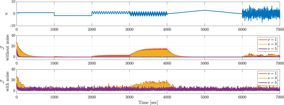
Figure 3: Simulation results for the clamped beam system. The top figure depicts the input signal, while the middle and bottom figures depict the performance measure(16) for the simulations without and with noise, respectively.

The middle plot of Figure3 depicts 𝒥\mathcal{J}caligraphic_J. It can be concluded that all low-dimensional observers converge exponentially fast to the system state for constant inputs, i.e., up to t=2​T t=2T italic_t = 2 italic_T. This is expected, as 0 is an interpolation point in all observer designs. Next, for 2​T<t≤3​T 2T<t\leq 3T 2 italic_T < italic_t ≤ 3 italic_T, the input is a sine wave with frequency ω 1\omega_{1}italic_ω start_POSTSUBSCRIPT 1 end_POSTSUBSCRIPT. As this frequency is matched in both the ν=3\nu=3 italic_ν = 3 and ν=5\nu=5 italic_ν = 5 case, these observers provide again convergence to zero error. However, the observer corresponding to ν=1\nu=1 italic_ν = 1, which does not match this frequency, yields a periodic error with frequency ω 1\omega_{1}italic_ω start_POSTSUBSCRIPT 1 end_POSTSUBSCRIPT. Next, for 3​T<t≤4​T 3T<t\leq 4T 3 italic_T < italic_t ≤ 4 italic_T, the input is constituted of two sine waves with the frequencies ω 1\omega_{1}italic_ω start_POSTSUBSCRIPT 1 end_POSTSUBSCRIPT and ω 2\omega_{2}italic_ω start_POSTSUBSCRIPT 2 end_POSTSUBSCRIPT. It can be seen that only the observer corresponding to ν=5\nu=5 italic_ν = 5 yields zero error. The other two observers give a non-zero error. Next, from 4​T<t≤6​T 4T<t\leq 6T 4 italic_T < italic_t ≤ 6 italic_T, the input is an increasing and decreasing ramp. Since this ramp is sufficiently slow, all observers achieve an error close to zero. Finally, when the input is a white-noise sequence, all errors are non-zero. In conclusion, this example demonstrates the role of the interpolation points in the estimation error of the observers. In particular, it is shown that full-state estimation can be achieved for certain classes of inputs.

Consider now the case in which the system output y y italic_y is polluted with a zero-order-hold realization of a zero-mean white noise sequence with a variance that corresponds to a signal-to-noise ratio (SNR) of 1 1 1 The SNR is defined as SNR=10​log 10⁡((y−μ)⊤​(y−μ)η⊤​η)\text{SNR}=10\log_{10}\left(\frac{(y-\mu)^{\top}(y-\mu)}{\eta^{\top}\eta}\right)SNR = 10 roman_log start_POSTSUBSCRIPT 10 end_POSTSUBSCRIPT ( divide start_ARG ( italic_y - italic_μ ) start_POSTSUPERSCRIPT ⊤ end_POSTSUPERSCRIPT ( italic_y - italic_μ ) end_ARG start_ARG italic_η start_POSTSUPERSCRIPT ⊤ end_POSTSUPERSCRIPT italic_η end_ARG ), where y y italic_y represent the sequence of {y​(t k)}k=0 N{y(t_{k})}{k=0}^{N}{ italic_y ( italic_t start_POSTSUBSCRIPT italic_k end_POSTSUBSCRIPT ) } start_POSTSUBSCRIPT italic_k = 0 end_POSTSUBSCRIPT start_POSTSUPERSCRIPT italic_N end_POSTSUPERSCRIPT at samples t k t{k}italic_t start_POSTSUBSCRIPT italic_k end_POSTSUBSCRIPT and μ\mu italic_μ is the mean of this sequence, and where η\eta italic_η is the white-noise sequence {η​(t k)}k=0 N{\eta(t_{k})}_{k=0}^{N}{ italic_η ( italic_t start_POSTSUBSCRIPT italic_k end_POSTSUBSCRIPT ) } start_POSTSUBSCRIPT italic_k = 0 end_POSTSUBSCRIPT start_POSTSUPERSCRIPT italic_N end_POSTSUPERSCRIPT. 20 dB. The bottom plot of Figure3 shows the performance measure 𝒥\mathcal{J}caligraphic_J, from which we conclude that the estimation error does not converge to exactly zero, but remains close to zero. This error is consistent for all observers, except at the interval 3​T<t≤4​T 3T<t\leq 4T 3 italic_T < italic_t ≤ 4 italic_T, where the observers corresponding to ν=1\nu=1 italic_ν = 1 and ν=3\nu=3 italic_ν = 3 exhibit an error similar to the case without noise.

VI Conclusions

This article presents a low-dimensional observer design approach for single-input single-output stable linear time-invariant systems. We have exploited recent advances in model order reduction for this purpose [14]. In particular, the approach consists in first deriving a reduced-order model of the plant dynamics for a given class of inputs. An observer is then designed based on this reduced-order model, which generates estimates that are used to reconstruct the original full state of the plant model. The results are demonstrated in a simulation on a benchmark model reduction problem.

In future work, we will extend the presented results to systems with possibly unstable state matrices and output nonlinearities thereby opening the door to the application to, e.g., lithium-ion battery models like those in [3, 4, 2].

Proof of Proposition2

Let e=(e x​ω,e ξ^​ω)∈ℝ n×ℝ ν e=(e_{x\omega},e_{\hat{\xi}\omega})\in\mathbb{R}^{n}\times\mathbb{R}^{\nu}italic_e = ( italic_e start_POSTSUBSCRIPT italic_x italic_ω end_POSTSUBSCRIPT , italic_e start_POSTSUBSCRIPT over^ start_ARG italic_ξ end_ARG italic_ω end_POSTSUBSCRIPT ) ∈ blackboard_R start_POSTSUPERSCRIPT italic_n end_POSTSUPERSCRIPT × blackboard_R start_POSTSUPERSCRIPT italic_ν end_POSTSUPERSCRIPT and Q≻0 Q\succ 0 italic_Q ≻ 0. As Ξ\Xi roman_Ξ is a Hurwitz matrix by assumption, there exists a unique P≻0 P\succ 0 italic_P ≻ 0 such that P​Ξ+Ξ⊤​P=−Q P\Xi+\Xi^{\top}P=-Q italic_P roman_Ξ + roman_Ξ start_POSTSUPERSCRIPT ⊤ end_POSTSUPERSCRIPT italic_P = - italic_Q. We consider the Lyapunov function candidate V​(e):=e⊤​P​e V(e):=e^{\top}Pe italic_V ( italic_e ) := italic_e start_POSTSUPERSCRIPT ⊤ end_POSTSUPERSCRIPT italic_P italic_e for any e∈ℝ n+ν e\in\mathbb{R}^{n+\nu}italic_e ∈ blackboard_R start_POSTSUPERSCRIPT italic_n + italic_ν end_POSTSUPERSCRIPT. In view of (IV-A), we have

⟨∇V​(e),Ξ​e+Ψ​(u−L​ω)⟩=e⊤​(P​Ξ+Ξ⊤​P)​e+2​e⊤​P​Ψ​(u−L​ω).\langle\nabla V(e),\Xi e+\Psi(u-L\omega)\rangle\ =e^{\top}(P\Xi+\Xi^{\top}P)e+2e^{\top}P\Psi(u-L\omega).start_ROW start_CELL ⟨ ∇ italic_V ( italic_e ) , roman_Ξ italic_e + roman_Ψ ( italic_u - italic_L italic_ω ) ⟩ end_CELL end_ROW start_ROW start_CELL = italic_e start_POSTSUPERSCRIPT ⊤ end_POSTSUPERSCRIPT ( italic_P roman_Ξ + roman_Ξ start_POSTSUPERSCRIPT ⊤ end_POSTSUPERSCRIPT italic_P ) italic_e + 2 italic_e start_POSTSUPERSCRIPT ⊤ end_POSTSUPERSCRIPT italic_P roman_Ψ ( italic_u - italic_L italic_ω ) . end_CELL end_ROW(17)

By definition of P P italic_P and the Cauchy-Schwarz inequality,

⟨∇V​(e),Ξ​e+Ψ​(u−L​ω)⟩≤−e⊤​Q​e+2​‖e‖​‖P​Ψ‖​‖u−L​ω‖.\langle\nabla V(e),\Xi e+\Psi(u-L\omega)\rangle\ \leq-e^{\top}Qe+2|e||P\Psi||u-L\omega|.start_ROW start_CELL ⟨ ∇ italic_V ( italic_e ) , roman_Ξ italic_e + roman_Ψ ( italic_u - italic_L italic_ω ) ⟩ end_CELL end_ROW start_ROW start_CELL ≤ - italic_e start_POSTSUPERSCRIPT ⊤ end_POSTSUPERSCRIPT italic_Q italic_e + 2 ∥ italic_e ∥ ∥ italic_P roman_Ψ ∥ ∥ italic_u - italic_L italic_ω ∥ . end_CELL end_ROW(18)

Using the fact that for any p 1 p_{1}italic_p start_POSTSUBSCRIPT 1 end_POSTSUBSCRIPT, p 2∈ℝ≥0 p_{2}\in\mathbb{R}{\geq 0}italic_p start_POSTSUBSCRIPT 2 end_POSTSUBSCRIPT ∈ blackboard_R start_POSTSUBSCRIPT ≥ 0 end_POSTSUBSCRIPT and η∈ℝ>0\eta\in\mathbb{R}{>0}italic_η ∈ blackboard_R start_POSTSUBSCRIPT > 0 end_POSTSUBSCRIPT, 2​p 1​p 2≤η 2​p 1 2+2 η​p 2 2 2p_{1}p_{2}\leq\tfrac{\eta}{2}p_{1}^{2}+\tfrac{2}{\eta}p_{2}^{2}2 italic_p start_POSTSUBSCRIPT 1 end_POSTSUBSCRIPT italic_p start_POSTSUBSCRIPT 2 end_POSTSUBSCRIPT ≤ divide start_ARG italic_η end_ARG start_ARG 2 end_ARG italic_p start_POSTSUBSCRIPT 1 end_POSTSUBSCRIPT start_POSTSUPERSCRIPT 2 end_POSTSUPERSCRIPT + divide start_ARG 2 end_ARG start_ARG italic_η end_ARG italic_p start_POSTSUBSCRIPT 2 end_POSTSUBSCRIPT start_POSTSUPERSCRIPT 2 end_POSTSUPERSCRIPT, by taking p 1=‖e‖p_{1}=|e|italic_p start_POSTSUBSCRIPT 1 end_POSTSUBSCRIPT = ∥ italic_e ∥, p 2=‖P​Ψ‖​‖u−L​ω‖p_{2}=|P\Psi||u-L\omega|italic_p start_POSTSUBSCRIPT 2 end_POSTSUBSCRIPT = ∥ italic_P roman_Ψ ∥ ∥ italic_u - italic_L italic_ω ∥, and η=λ min​(Q)\eta=\lambda_{\min}(Q)italic_η = italic_λ start_POSTSUBSCRIPT roman_min end_POSTSUBSCRIPT ( italic_Q ), we obtain

⟨∇\displaystyle\langle\nabla⟨ ∇V(e),Ξ e+Ψ(u−L ω)⟩\displaystyle V(e),\Xi e+\Psi(u-L\omega)\rangle italic_V ( italic_e ) , roman_Ξ italic_e + roman_Ψ ( italic_u - italic_L italic_ω ) ⟩ ≤−λ min​(Q)​‖e‖2+λ min​(Q)2​‖e‖2+2​‖P​Ψ‖2 λ min​(Q)​‖u−L​ω‖2\displaystyle\leq-\lambda_{\min}(Q)|e|^{2}+\tfrac{\lambda_{\min}(Q)}{2}|e|^{2}+\tfrac{2|P\Psi|^{2}}{\lambda_{\min}(Q)}|u-L\omega|^{2}≤ - italic_λ start_POSTSUBSCRIPT roman_min end_POSTSUBSCRIPT ( italic_Q ) ∥ italic_e ∥ start_POSTSUPERSCRIPT 2 end_POSTSUPERSCRIPT + divide start_ARG italic_λ start_POSTSUBSCRIPT roman_min end_POSTSUBSCRIPT ( italic_Q ) end_ARG start_ARG 2 end_ARG ∥ italic_e ∥ start_POSTSUPERSCRIPT 2 end_POSTSUPERSCRIPT + divide start_ARG 2 ∥ italic_P roman_Ψ ∥ start_POSTSUPERSCRIPT 2 end_POSTSUPERSCRIPT end_ARG start_ARG italic_λ start_POSTSUBSCRIPT roman_min end_POSTSUBSCRIPT ( italic_Q ) end_ARG ∥ italic_u - italic_L italic_ω ∥ start_POSTSUPERSCRIPT 2 end_POSTSUPERSCRIPT ≤−λ min​(Q)2​‖e‖2+2​‖P​Ψ‖2 λ min​(Q)​‖u−L​ω‖2.\displaystyle\leq-\tfrac{\lambda_{\min}(Q)}{2}|e|^{2}+\tfrac{2|P\Psi|^{2}}{\lambda_{\min}(Q)}|u-L\omega|^{2}.≤ - divide start_ARG italic_λ start_POSTSUBSCRIPT roman_min end_POSTSUBSCRIPT ( italic_Q ) end_ARG start_ARG 2 end_ARG ∥ italic_e ∥ start_POSTSUPERSCRIPT 2 end_POSTSUPERSCRIPT + divide start_ARG 2 ∥ italic_P roman_Ψ ∥ start_POSTSUPERSCRIPT 2 end_POSTSUPERSCRIPT end_ARG start_ARG italic_λ start_POSTSUBSCRIPT roman_min end_POSTSUBSCRIPT ( italic_Q ) end_ARG ∥ italic_u - italic_L italic_ω ∥ start_POSTSUPERSCRIPT 2 end_POSTSUPERSCRIPT .(19)

Using (19) and λ min​(P)​‖e‖2≤V​(e)≤λ max​(P)​‖e‖2\lambda_{\min}(P)|e|^{2}\leq V(e)\leq\lambda_{\max}(P)|e|^{2}italic_λ start_POSTSUBSCRIPT roman_min end_POSTSUBSCRIPT ( italic_P ) ∥ italic_e ∥ start_POSTSUPERSCRIPT 2 end_POSTSUPERSCRIPT ≤ italic_V ( italic_e ) ≤ italic_λ start_POSTSUBSCRIPT roman_max end_POSTSUBSCRIPT ( italic_P ) ∥ italic_e ∥ start_POSTSUPERSCRIPT 2 end_POSTSUPERSCRIPT, we derive (11) with c 1:=‖Φ‖​λ max​(P)λ min​(P)c_{1}:=|\Phi|\sqrt{\tfrac{\lambda_{\max}(P)}{\lambda_{\min}(P)}}italic_c start_POSTSUBSCRIPT 1 end_POSTSUBSCRIPT := ∥ roman_Φ ∥ square-root start_ARG divide start_ARG italic_λ start_POSTSUBSCRIPT roman_max end_POSTSUBSCRIPT ( italic_P ) end_ARG start_ARG italic_λ start_POSTSUBSCRIPT roman_min end_POSTSUBSCRIPT ( italic_P ) end_ARG end_ARG, c 2:=λ min​(Q)4​λ max​(P)c_{2}:=\tfrac{\lambda_{\min}(Q)}{4\lambda_{\max}(P)}italic_c start_POSTSUBSCRIPT 2 end_POSTSUBSCRIPT := divide start_ARG italic_λ start_POSTSUBSCRIPT roman_min end_POSTSUBSCRIPT ( italic_Q ) end_ARG start_ARG 4 italic_λ start_POSTSUBSCRIPT roman_max end_POSTSUBSCRIPT ( italic_P ) end_ARG, c 3:=2​‖Φ‖​‖P​Ψ‖λ min​(Q)​λ max​(P)λ min​(P)c_{3}:=\tfrac{2|\Phi||P\Psi|}{\lambda_{\min}(Q)}\sqrt{\tfrac{\lambda_{\max}(P)}{\lambda_{\min}(P)}}italic_c start_POSTSUBSCRIPT 3 end_POSTSUBSCRIPT := divide start_ARG 2 ∥ roman_Φ ∥ ∥ italic_P roman_Ψ ∥ end_ARG start_ARG italic_λ start_POSTSUBSCRIPT roman_min end_POSTSUBSCRIPT ( italic_Q ) end_ARG square-root start_ARG divide start_ARG italic_λ start_POSTSUBSCRIPT roman_max end_POSTSUBSCRIPT ( italic_P ) end_ARG start_ARG italic_λ start_POSTSUBSCRIPT roman_min end_POSTSUBSCRIPT ( italic_P ) end_ARG end_ARG, and Φ\Phi roman_Φ the matrix in (IV-A) by following similar lines as in the proof of [21, Theorem 4.10].

References

• [1] P.Bernard, V.Andrieu, and D.Astolfi, “Observer design for continuous-time dynamical systems,” Annual Reviews in Control, vol.53, pp.224–248, 2022.
• [2] S.Dey and B.Ayalew, “Nonlinear observer designs for state-of-charge estimation of lithium-ion batteries,” in IEEE American Control Conference, Portland, USA, pp.248–253, 2014.
• [3] P.G. Blondel, R.Postoyan, S.Raël, S.Benjamin, and P.Desprez, “Nonlinear circle-criterion observer design for an electrochemical battery model,” IEEE Transactions on Control Systems Technology, vol.27, no.2, pp.889–897, 2018.
• [4] M.Khalil, R.Postoyan, and S.Raël, “Enhancing accuracy of finite-dimensional models for lithium-ion batteries, observer design, and experimental validation,” IEEE Transactions on Control Systems Technology, vol.33, no.1, pp.327 – 342, 2024.
• [5] M.Khalil, R.Postoyan, S.Raël, and D.Nešić, “Hybrid low-dimensional limiting state of charge estimator for multi-cell lithium-ion batteries,” in IEEE Conference on Decision and Control, Milan, Italy, 2024.
• [6] M.Darouach, M.Zasadzinski, and M.Hayar, “Reduced-order observer design for descriptor systems with unknown inputs,” IEEE Transactions on Automatic Control, vol.41, no.7, pp.1068–1072, 2002.
• [7] A.Astolfi, D.Karagiannis, and R.Ortega, Nonlinear and Adaptive Control with Applications. New York, USA: Springer, 2008.
• [8] M.Arcak and P.Kokotović, “Nonlinear observers: a circle criterion design and robustness analysis,” Automatica, vol.37, pp.1923–1930, 2001.
• [9] T.Sadamoto, T.Ishizaki, and J.-i. Imura, “Low-dimensional functional observer design for linear systems via observer reduction approach,” in IEEE Conference on Decision and Control, Florence, Italy, pp.776–781, 2013.
• [10] W.Han, H.Trentelman, Z.Wang, and Y.Shen, “A simple approach to distributed observer design for linear systems,” IEEE Transactions on Automatic Control, vol.64, no.1, pp.329–336, 2018.
• [11] L.Wang and A.Morse, “A distributed observer for a time-invariant linear system,” IEEE Transactions on Automatic Control, vol.63, no.7, pp.2123–2130, 2017.
• [12] T.Sadamoto, T.Ishizaki, and J.-i. Imura, “Average state observers for large-scale network systems,” IEEE Transactions on Control of Network Systems, vol.4, no.4, pp.761–769, 2016.
• [13] G.Plett, “Efficient battery pack state estimation using bar-delta filtering,” in EVS24 International Battery, Hybrid and Fuel Cell Electric Vehicle Symposium, Stavenger, Norway, pp.1–8, 2009.
• [14] A.Astolfi, “Model reduction by moment matching for linear and nonlinear systems,” IEEE Transactions on Automatic Control, vol.55, no.10, pp.2321–2336, 2010.
• [15] J.P. Hespanha, Linear Systems Theory: Second Edition. Princeton University Press, New Jersey, 2018.
• [16] E.de Souza and S.P. Bhattacharyya, “Controllability, observability and the solution of A​X−X​B=C AX-XB=C italic_A italic_X - italic_X italic_B = italic_C,” Linear Algebra and its Applications, vol.39, pp.167–188, 1981.
• [17] M.F. Shakib, G.Scarciotti, M.Jungers, A.Pogromsky, A.Pavlov, and N.van de Wouw, “Optimal ℋ∞\mathcal{H}_{\infty}caligraphic_H start_POSTSUBSCRIPT ∞ end_POSTSUBSCRIPT LMI-Based Model Reduction by Moment Matching for Linear Time-Invariant Models,” in IEEE Conference on Decision and Control, Austin, USA, pp.6914–6919, 2021.
• [18] F.Shakib, G.Scarciotti, M.Jungers, A.Y. Pogromsky, A.Pavlov, and N.van de Wouw, “Optimal model reduction by time-domain moment matching for Lur’e-type models,” IEEE Transactions on Automatic Control, pp.1–8, 2024.
• [19] G.Scarciotti and A.Astolfi, “Interconnection-based model order reduction - a survey,” European Journal of Control, vol.75, p.100929, 2024.
• [20] A.C. Antoulas, D.C. Sorensen, and S.Gugercin, “A survey of model reduction methods for large-scale systems,” Contemporary Mathematics, vol.280, pp.193–220, 2001.
• [21] H.K. Khalil, Nonlinear Systems. Prentice-Hall, Third Edition, New Jersey, USA, 2002.