Spaces:
Running

Running

| """ | |
| Title: Monocular depth estimation | |
| Author: [Victor Basu](https://www.linkedin.com/in/victor-basu-520958147) | |
| Date created: 2021/08/30 | |
| Last modified: 2024/08/13 | |
| Description: Implement a depth estimation model with a convnet. | |
| Accelerator: GPU | |
| """ | |
| """ | |
| ## Introduction | |
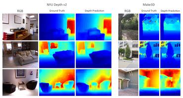
| _Depth estimation_ is a crucial step towards inferring scene geometry from 2D images. | |
| The goal in _monocular depth estimation_ is to predict the depth value of each pixel or | |
| inferring depth information, given only a single RGB image as input. | |
| This example will show an approach to build a depth estimation model with a convnet | |
| and simple loss functions. | |
|  | |
| """ | |
| """ | |
| ## Setup | |
| """ | |
| import os | |
| os.environ["KERAS_BACKEND"] = "tensorflow" | |
| import sys | |
| import tensorflow as tf | |
| import keras | |
| from keras import layers | |
| from keras import ops | |
| import pandas as pd | |
| import numpy as np | |
| import cv2 | |
| import matplotlib.pyplot as plt | |
| keras.utils.set_random_seed(123) | |
| """ | |
| ## Downloading the dataset | |
| We will be using the dataset **DIODE: A Dense Indoor and Outdoor Depth Dataset** for this | |
| tutorial. However, we use the validation set generating training and evaluation subsets | |
| for our model. The reason we use the validation set rather than the training set of the original dataset is because | |
| the training set consists of 81GB of data, which is challenging to download compared | |
| to the validation set which is only 2.6GB. | |
| Other datasets that you could use are | |
| **[NYU-v2](https://cs.nyu.edu/~silberman/datasets/nyu_depth_v2.html)** | |
| and **[KITTI](http://www.cvlibs.net/datasets/kitti/)**. | |
| """ | |
| annotation_folder = "/dataset/" | |
| if not os.path.exists(os.path.abspath(".") + annotation_folder): | |
| annotation_zip = keras.utils.get_file( | |
| "val.tar.gz", | |
| cache_subdir=os.path.abspath("."), | |
| origin="http://diode-dataset.s3.amazonaws.com/val.tar.gz", | |
| extract=True, | |
| ) | |
| """ | |
| ## Preparing the dataset | |
| We only use the indoor images to train our depth estimation model. | |
| """ | |
| path = "val/indoors" | |
| filelist = [] | |
| for root, dirs, files in os.walk(path): | |
| for file in files: | |
| filelist.append(os.path.join(root, file)) | |
| filelist.sort() | |
| data = { | |
| "image": [x for x in filelist if x.endswith(".png")], | |
| "depth": [x for x in filelist if x.endswith("_depth.npy")], | |
| "mask": [x for x in filelist if x.endswith("_depth_mask.npy")], | |
| } | |
| df = pd.DataFrame(data) | |
| df = df.sample(frac=1, random_state=42) | |
| """ | |
| ## Preparing hyperparameters | |
| """ | |
| HEIGHT = 256 | |
| WIDTH = 256 | |
| LR = 0.00001 | |
| EPOCHS = 30 | |
| BATCH_SIZE = 32 | |
| """ | |
| ## Building a data pipeline | |
| 1. The pipeline takes a dataframe containing the path for the RGB images, | |
| as well as the depth and depth mask files. | |
| 2. It reads and resize the RGB images. | |
| 3. It reads the depth and depth mask files, process them to generate the depth map image and | |
| resize it. | |
| 4. It returns the RGB images and the depth map images for a batch. | |
| """ | |
| class DataGenerator(keras.utils.PyDataset): | |
| def __init__(self, data, batch_size=6, dim=(768, 1024), n_channels=3, shuffle=True): | |
| super().__init__() | |
| """ | |
| Initialization | |
| """ | |
| self.data = data | |
| self.indices = self.data.index.tolist() | |
| self.dim = dim | |
| self.n_channels = n_channels | |
| self.batch_size = batch_size | |
| self.shuffle = shuffle | |
| self.min_depth = 0.1 | |
| self.on_epoch_end() | |
| def __len__(self): | |
| return int(np.ceil(len(self.data) / self.batch_size)) | |
| def __getitem__(self, index): | |
| if (index + 1) * self.batch_size > len(self.indices): | |
| self.batch_size = len(self.indices) - index * self.batch_size | |
| # Generate one batch of data | |
| # Generate indices of the batch | |
| index = self.indices[index * self.batch_size : (index + 1) * self.batch_size] | |
| # Find list of IDs | |
| batch = [self.indices[k] for k in index] | |
| x, y = self.data_generation(batch) | |
| return x, y | |
| def on_epoch_end(self): | |
| """ | |
| Updates indexes after each epoch | |
| """ | |
| self.index = np.arange(len(self.indices)) | |
| if self.shuffle == True: | |
| np.random.shuffle(self.index) | |
| def load(self, image_path, depth_map, mask): | |
| """Load input and target image.""" | |
| image_ = cv2.imread(image_path) | |
| image_ = cv2.cvtColor(image_, cv2.COLOR_BGR2RGB) | |
| image_ = cv2.resize(image_, self.dim) | |
| image_ = tf.image.convert_image_dtype(image_, tf.float32) | |
| depth_map = np.load(depth_map).squeeze() | |
| mask = np.load(mask) | |
| mask = mask > 0 | |
| max_depth = min(300, np.percentile(depth_map, 99)) | |
| depth_map = np.clip(depth_map, self.min_depth, max_depth) | |
| depth_map = np.log(depth_map, where=mask) | |
| depth_map = np.ma.masked_where(~mask, depth_map) | |
| depth_map = np.clip(depth_map, 0.1, np.log(max_depth)) | |
| depth_map = cv2.resize(depth_map, self.dim) | |
| depth_map = np.expand_dims(depth_map, axis=2) | |
| depth_map = tf.image.convert_image_dtype(depth_map, tf.float32) | |
| return image_, depth_map | |
| def data_generation(self, batch): | |
| x = np.empty((self.batch_size, *self.dim, self.n_channels)) | |
| y = np.empty((self.batch_size, *self.dim, 1)) | |
| for i, batch_id in enumerate(batch): | |
| x[i,], y[i,] = self.load( | |
| self.data["image"][batch_id], | |
| self.data["depth"][batch_id], | |
| self.data["mask"][batch_id], | |
| ) | |
| x, y = x.astype("float32"), y.astype("float32") | |
| return x, y | |
| """ | |
| ## Visualizing samples | |
| """ | |
| def visualize_depth_map(samples, test=False, model=None): | |
| input, target = samples | |
| cmap = plt.cm.jet | |
| cmap.set_bad(color="black") | |
| if test: | |
| pred = model.predict(input) | |
| fig, ax = plt.subplots(6, 3, figsize=(50, 50)) | |
| for i in range(6): | |
| ax[i, 0].imshow((input[i].squeeze())) | |
| ax[i, 1].imshow((target[i].squeeze()), cmap=cmap) | |
| ax[i, 2].imshow((pred[i].squeeze()), cmap=cmap) | |
| else: | |
| fig, ax = plt.subplots(6, 2, figsize=(50, 50)) | |
| for i in range(6): | |
| ax[i, 0].imshow((input[i].squeeze())) | |
| ax[i, 1].imshow((target[i].squeeze()), cmap=cmap) | |
| visualize_samples = next( | |
| iter(DataGenerator(data=df, batch_size=6, dim=(HEIGHT, WIDTH))) | |
| ) | |
| visualize_depth_map(visualize_samples) | |
| """ | |
| ## 3D point cloud visualization | |
| """ | |
| depth_vis = np.flipud(visualize_samples[1][1].squeeze()) # target | |
| img_vis = np.flipud(visualize_samples[0][1].squeeze()) # input | |
| fig = plt.figure(figsize=(15, 10)) | |
| ax = plt.axes(projection="3d") | |
| STEP = 3 | |
| for x in range(0, img_vis.shape[0], STEP): | |
| for y in range(0, img_vis.shape[1], STEP): | |
| ax.scatter( | |
| [depth_vis[x, y]] * 3, | |
| [y] * 3, | |
| [x] * 3, | |
| c=tuple(img_vis[x, y, :3] / 255), | |
| s=3, | |
| ) | |
| ax.view_init(45, 135) | |
| """ | |
| ## Building the model | |
| 1. The basic model is from U-Net. | |
| 2. Addditive skip-connections are implemented in the downscaling block. | |
| """ | |
| class DownscaleBlock(layers.Layer): | |
| def __init__( | |
| self, filters, kernel_size=(3, 3), padding="same", strides=1, **kwargs | |
| ): | |
| super().__init__(**kwargs) | |
| self.convA = layers.Conv2D(filters, kernel_size, strides, padding) | |
| self.convB = layers.Conv2D(filters, kernel_size, strides, padding) | |
| self.reluA = layers.LeakyReLU(negative_slope=0.2) | |
| self.reluB = layers.LeakyReLU(negative_slope=0.2) | |
| self.bn2a = layers.BatchNormalization() | |
| self.bn2b = layers.BatchNormalization() | |
| self.pool = layers.MaxPool2D((2, 2), (2, 2)) | |
| def call(self, input_tensor): | |
| d = self.convA(input_tensor) | |
| x = self.bn2a(d) | |
| x = self.reluA(x) | |
| x = self.convB(x) | |
| x = self.bn2b(x) | |
| x = self.reluB(x) | |
| x += d | |
| p = self.pool(x) | |
| return x, p | |
| class UpscaleBlock(layers.Layer): | |
| def __init__( | |
| self, filters, kernel_size=(3, 3), padding="same", strides=1, **kwargs | |
| ): | |
| super().__init__(**kwargs) | |
| self.us = layers.UpSampling2D((2, 2)) | |
| self.convA = layers.Conv2D(filters, kernel_size, strides, padding) | |
| self.convB = layers.Conv2D(filters, kernel_size, strides, padding) | |
| self.reluA = layers.LeakyReLU(negative_slope=0.2) | |
| self.reluB = layers.LeakyReLU(negative_slope=0.2) | |
| self.bn2a = layers.BatchNormalization() | |
| self.bn2b = layers.BatchNormalization() | |
| self.conc = layers.Concatenate() | |
| def call(self, x, skip): | |
| x = self.us(x) | |
| concat = self.conc([x, skip]) | |
| x = self.convA(concat) | |
| x = self.bn2a(x) | |
| x = self.reluA(x) | |
| x = self.convB(x) | |
| x = self.bn2b(x) | |
| x = self.reluB(x) | |
| return x | |
| class BottleNeckBlock(layers.Layer): | |
| def __init__( | |
| self, filters, kernel_size=(3, 3), padding="same", strides=1, **kwargs | |
| ): | |
| super().__init__(**kwargs) | |
| self.convA = layers.Conv2D(filters, kernel_size, strides, padding) | |
| self.convB = layers.Conv2D(filters, kernel_size, strides, padding) | |
| self.reluA = layers.LeakyReLU(negative_slope=0.2) | |
| self.reluB = layers.LeakyReLU(negative_slope=0.2) | |
| def call(self, x): | |
| x = self.convA(x) | |
| x = self.reluA(x) | |
| x = self.convB(x) | |
| x = self.reluB(x) | |
| return x | |
| """ | |
| ## Defining the loss | |
| We will optimize 3 losses in our mode. | |
| 1. Structural similarity index(SSIM). | |
| 2. L1-loss, or Point-wise depth in our case. | |
| 3. Depth smoothness loss. | |
| Out of the three loss functions, SSIM contributes the most to improving model performance. | |
| """ | |
| def image_gradients(image): | |
| if len(ops.shape(image)) != 4: | |
| raise ValueError( | |
| "image_gradients expects a 4D tensor " | |
| "[batch_size, h, w, d], not {}.".format(ops.shape(image)) | |
| ) | |
| image_shape = ops.shape(image) | |
| batch_size, height, width, depth = ops.unstack(image_shape) | |
| dy = image[:, 1:, :, :] - image[:, :-1, :, :] | |
| dx = image[:, :, 1:, :] - image[:, :, :-1, :] | |
| # Return tensors with same size as original image by concatenating | |
| # zeros. Place the gradient [I(x+1,y) - I(x,y)] on the base pixel (x, y). | |
| shape = ops.stack([batch_size, 1, width, depth]) | |
| dy = ops.concatenate([dy, ops.zeros(shape, dtype=image.dtype)], axis=1) | |
| dy = ops.reshape(dy, image_shape) | |
| shape = ops.stack([batch_size, height, 1, depth]) | |
| dx = ops.concatenate([dx, ops.zeros(shape, dtype=image.dtype)], axis=2) | |
| dx = ops.reshape(dx, image_shape) | |
| return dy, dx | |
| class DepthEstimationModel(keras.Model): | |
| def __init__(self): | |
| super().__init__() | |
| self.ssim_loss_weight = 0.85 | |
| self.l1_loss_weight = 0.1 | |
| self.edge_loss_weight = 0.9 | |
| self.loss_metric = keras.metrics.Mean(name="loss") | |
| f = [16, 32, 64, 128, 256] | |
| self.downscale_blocks = [ | |
| DownscaleBlock(f[0]), | |
| DownscaleBlock(f[1]), | |
| DownscaleBlock(f[2]), | |
| DownscaleBlock(f[3]), | |
| ] | |
| self.bottle_neck_block = BottleNeckBlock(f[4]) | |
| self.upscale_blocks = [ | |
| UpscaleBlock(f[3]), | |
| UpscaleBlock(f[2]), | |
| UpscaleBlock(f[1]), | |
| UpscaleBlock(f[0]), | |
| ] | |
| self.conv_layer = layers.Conv2D(1, (1, 1), padding="same", activation="tanh") | |
| def calculate_loss(self, target, pred): | |
| # Edges | |
| dy_true, dx_true = image_gradients(target) | |
| dy_pred, dx_pred = image_gradients(pred) | |
| weights_x = ops.cast(ops.exp(ops.mean(ops.abs(dx_true))), "float32") | |
| weights_y = ops.cast(ops.exp(ops.mean(ops.abs(dy_true))), "float32") | |
| # Depth smoothness | |
| smoothness_x = dx_pred * weights_x | |
| smoothness_y = dy_pred * weights_y | |
| depth_smoothness_loss = ops.mean(abs(smoothness_x)) + ops.mean( | |
| abs(smoothness_y) | |
| ) | |
| # Structural similarity (SSIM) index | |
| ssim_loss = ops.mean( | |
| 1 | |
| - tf.image.ssim( | |
| target, pred, max_val=WIDTH, filter_size=7, k1=0.01**2, k2=0.03**2 | |
| ) | |
| ) | |
| # Point-wise depth | |
| l1_loss = ops.mean(ops.abs(target - pred)) | |
| loss = ( | |
| (self.ssim_loss_weight * ssim_loss) | |
| + (self.l1_loss_weight * l1_loss) | |
| + (self.edge_loss_weight * depth_smoothness_loss) | |
| ) | |
| return loss | |
| def metrics(self): | |
| return [self.loss_metric] | |
| def train_step(self, batch_data): | |
| input, target = batch_data | |
| with tf.GradientTape() as tape: | |
| pred = self(input, training=True) | |
| loss = self.calculate_loss(target, pred) | |
| gradients = tape.gradient(loss, self.trainable_variables) | |
| self.optimizer.apply_gradients(zip(gradients, self.trainable_variables)) | |
| self.loss_metric.update_state(loss) | |
| return { | |
| "loss": self.loss_metric.result(), | |
| } | |
| def test_step(self, batch_data): | |
| input, target = batch_data | |
| pred = self(input, training=False) | |
| loss = self.calculate_loss(target, pred) | |
| self.loss_metric.update_state(loss) | |
| return { | |
| "loss": self.loss_metric.result(), | |
| } | |
| def call(self, x): | |
| c1, p1 = self.downscale_blocks[0](x) | |
| c2, p2 = self.downscale_blocks[1](p1) | |
| c3, p3 = self.downscale_blocks[2](p2) | |
| c4, p4 = self.downscale_blocks[3](p3) | |
| bn = self.bottle_neck_block(p4) | |
| u1 = self.upscale_blocks[0](bn, c4) | |
| u2 = self.upscale_blocks[1](u1, c3) | |
| u3 = self.upscale_blocks[2](u2, c2) | |
| u4 = self.upscale_blocks[3](u3, c1) | |
| return self.conv_layer(u4) | |
| """ | |
| ## Model training | |
| """ | |
| optimizer = keras.optimizers.SGD( | |
| learning_rate=LR, | |
| nesterov=False, | |
| ) | |
| model = DepthEstimationModel() | |
| # Compile the model | |
| model.compile(optimizer) | |
| train_loader = DataGenerator( | |
| data=df[:260].reset_index(drop="true"), batch_size=BATCH_SIZE, dim=(HEIGHT, WIDTH) | |
| ) | |
| validation_loader = DataGenerator( | |
| data=df[260:].reset_index(drop="true"), batch_size=BATCH_SIZE, dim=(HEIGHT, WIDTH) | |
| ) | |
| model.fit( | |
| train_loader, | |
| epochs=EPOCHS, | |
| validation_data=validation_loader, | |
| ) | |
| """ | |
| ## Visualizing model output | |
| We visualize the model output over the validation set. | |
| The first image is the RGB image, the second image is the ground truth depth map image | |
| and the third one is the predicted depth map image. | |
| """ | |
| test_loader = next( | |
| iter( | |
| DataGenerator( | |
| data=df[265:].reset_index(drop="true"), batch_size=6, dim=(HEIGHT, WIDTH) | |
| ) | |
| ) | |
| ) | |
| visualize_depth_map(test_loader, test=True, model=model) | |
| test_loader = next( | |
| iter( | |
| DataGenerator( | |
| data=df[300:].reset_index(drop="true"), batch_size=6, dim=(HEIGHT, WIDTH) | |
| ) | |
| ) | |
| ) | |
| visualize_depth_map(test_loader, test=True, model=model) | |
| """ | |
| ## Possible improvements | |
| 1. You can improve this model by replacing the encoding part of the U-Net with a | |
| pretrained DenseNet or ResNet. | |
| 2. Loss functions play an important role in solving this problem. | |
| Tuning the loss functions may yield significant improvement. | |
| """ | |
| """ | |
| ## References | |
| The following papers go deeper into possible approaches for depth estimation. | |
| 1. [Depth Prediction Without the Sensors: Leveraging Structure for Unsupervised Learning from Monocular Videos](https://arxiv.org/abs/1811.06152v1) | |
| 2. [Digging Into Self-Supervised Monocular Depth Estimation](https://openaccess.thecvf.com/content_ICCV_2019/papers/Godard_Digging_Into_Self-Supervised_Monocular_Depth_Estimation_ICCV_2019_paper.pdf) | |
| 3. [Deeper Depth Prediction with Fully Convolutional Residual Networks](https://arxiv.org/abs/1606.00373v2) | |
| You can also find helpful implementations in the papers with code depth estimation task. | |
| You can use the trained model hosted on [Hugging Face Hub](https://huggingface.co/spaces/keras-io/Monocular-Depth-Estimation) | |
| and try the demo on [Hugging Face Spaces](https://huggingface.co/keras-io/monocular-depth-estimation). | |
| """ | |