
Neural DNA (NDNA): A Compact Genome for Growing Network Architecture
A tiny learned genome (< 400 parameters) that grows neural network topology through developmental rules. Default disconnected, type-based compatibility, metabolic cost pressure. The genome discovers useful sparse connectivity that beats random wiring on every experiment (0.39% to 21.7%), matches or exceeds dense baselines on most, and transfers across tasks without retraining.
![]()
What is NDNA?
Neural networks typically use fixed, fully-connected layers. NDNA asks: what if a small "genome" could learn which connections should exist?
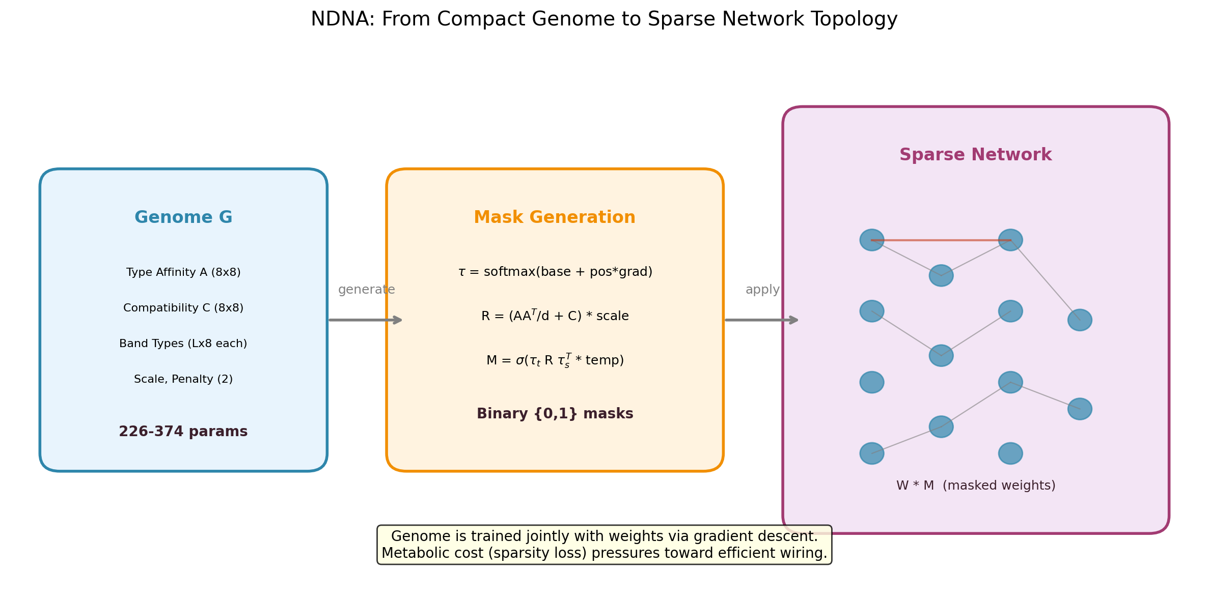
The genome encodes cell type embeddings and a compatibility matrix. During growth, it compares source and target types for every potential connection and decides whether to wire it or not. A metabolic cost penalty forces selectivity, so only useful connections survive.
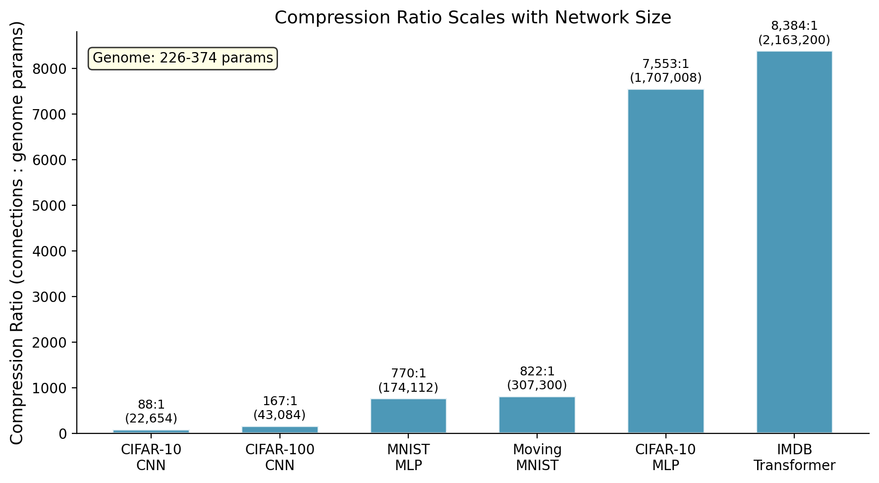
The result: 226 to 374 genome parameters control up to 2.2 million connections (8,384:1 compression on our benchmarks, likely higher on larger networks). The grown networks are sparse but structured, and they consistently beat randomly-wired sparse networks.
How It Works
- Genome encodes cell type embeddings (8 types, 8 dimensions) and a compatibility matrix
- Growth: for each potential connection, source and target type embeddings are compared via the compatibility matrix to produce a connection probability
- Binary mask: probabilities are thresholded to produce hard 0/1 masks (straight-through estimator for gradient flow)
- Metabolic cost: a sparsity loss penalizes total connection strength, forcing the genome to be selective
- Default disconnected: compatibility is initialized negative, so the genome must actively grow every connection
The genome and network weights are trained jointly with standard backpropagation.
Key Results
| Experiment | Genome | Random Sparse | Dense Baseline | Genome vs Random |
|---|---|---|---|---|
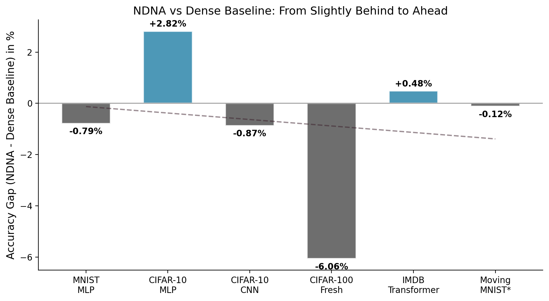
| MNIST (MLP) | 97.54% | 97.09% | 98.33% | +0.45% |
| CIFAR-10 (MLP) | 57.14% | 51.68% | 54.32% | +5.46% |
| CIFAR-10 (CNN) | 88.93% | 85.78% | 89.80% | +3.15% |
| CIFAR-100 (Transfer) | 60.92% | 53.91% | 67.16% | +7.01% |
| IMDB (Transformer) | 85.05% | 84.66% | 84.57% | +0.39% |
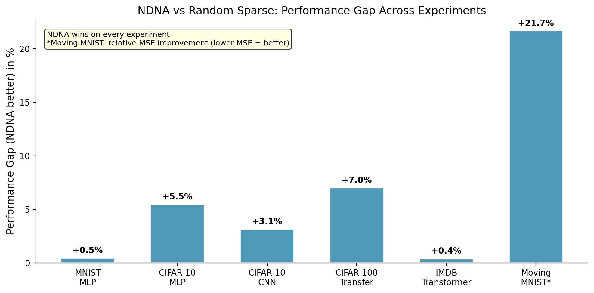
| Moving MNIST (Video)* | 62.23 | 79.44 | 62.15 | +21.7% |
*Moving MNIST uses MSE (lower is better). The +21.7% is relative improvement.
The genome beats random sparse wiring on every experiment. The largest gap is on video prediction (+21.7%), where random wiring completely falls apart but genome-grown wiring matches the dense baseline.
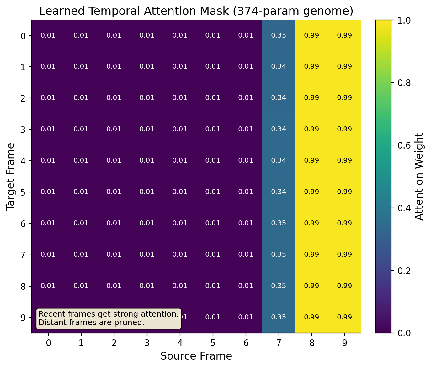
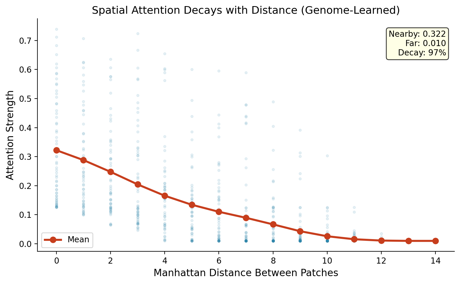
Video: Factored Spatiotemporal Genome
The video experiment uses a factored genome: temporal (74 params) + spatial (74 params) + depth (226 params) = 374 total. The temporal genome discovers temporal recency (recent frames get strong connections, distant frames get almost none). The spatial genome discovers spatial locality (nearby patches connect strongly, distant patches barely connect).
Pre-trained Genomes
These are the trained genome files. Each genome is tiny but controls the full network topology.
| File | Architecture | Task | Params | Connections | Compression | Result |
|---|---|---|---|---|---|---|
genome_mnist.pt |
MLP | MNIST | 226 | 174,240 | 770:1 | 97.54% |
genome_cifar10_mlp.pt |
MLP | CIFAR-10 | 226 | 1,706,240 | 7,553:1 | 57.14% |
genome_cifar10_cnn.pt |
CNN | CIFAR-10 | 258 | 165,888 | 643:1 | 88.93% |
genome_cifar100_fresh.pt |
MLP | CIFAR-100 (transfer) | 226 | 1,706,240 | 7,553:1 | 60.92% |
genome_transformer.pt |
Transformer | IMDB | 258 | 2,162,688 | 8,384:1 | 85.05% |
genome_video.pt |
Video Transformer | Moving MNIST | 374 | 307,300 | 821:1 | MSE 62.23 |
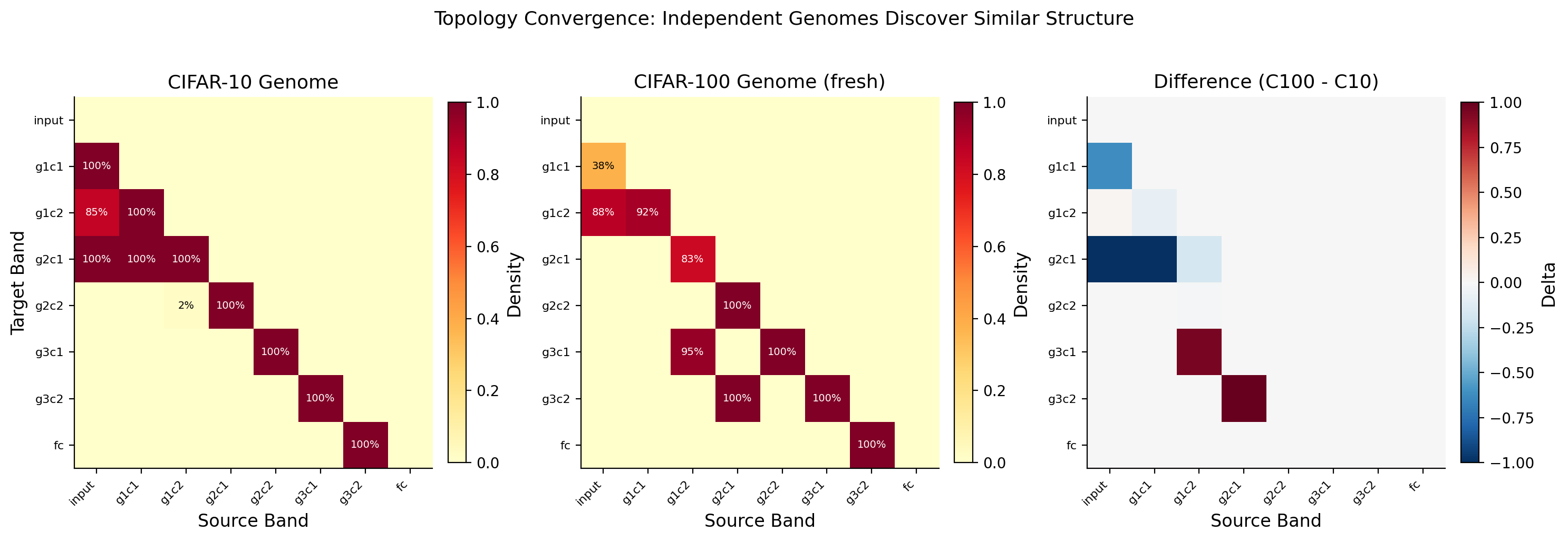
Cross-Task Transfer
The CIFAR-100 genome was not trained on CIFAR-100. It is the CIFAR-10 genome applied directly to CIFAR-100 without retraining the topology. Only the network weights were retrained. The genome's learned connectivity pattern transferred across tasks and still beat random sparse wiring by +7.01%.
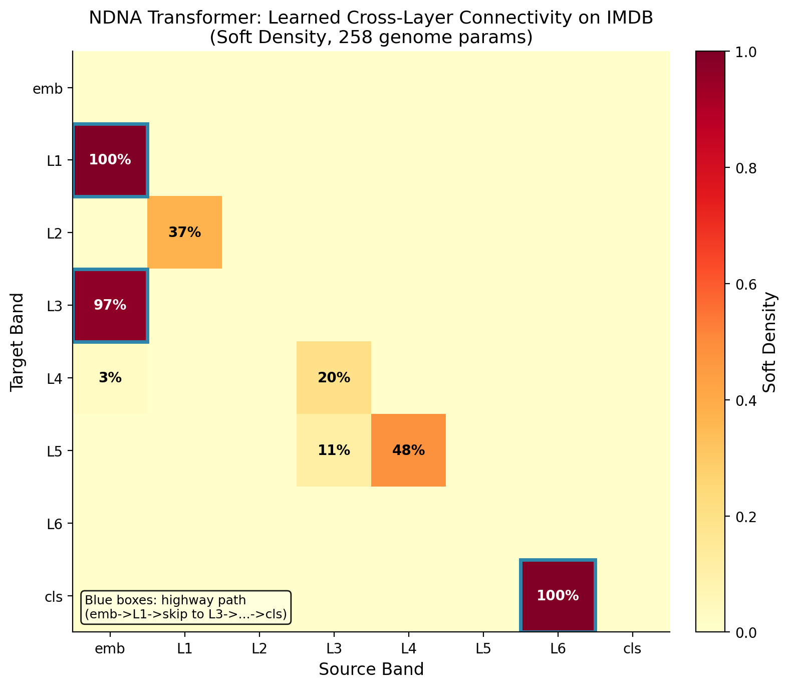
Transformer Attention Patterns
The genome also works on transformers. On IMDB sentiment analysis, the grown transformer beats both random sparse and dense baselines.
How to Use
import torch
from genome.model import Genome, GrownNetwork, GrownConvNetwork, GrownTransformer

# --- MLP (MNIST) ---
genome = Genome(n_types=8, type_dim=8, n_bands=6)
genome.load_state_dict(torch.load("genome_mnist.pt", weights_only=True))
model = GrownNetwork(genome, input_dim=784, hidden_bands=[48, 48, 48, 48], output_dim=10)

# --- MLP (CIFAR-10) ---
genome = Genome(n_types=8, type_dim=8, n_bands=6)
genome.load_state_dict(torch.load("genome_cifar10_mlp.pt", weights_only=True))
model = GrownNetwork(genome, input_dim=3072, hidden_bands=[128, 128, 128, 128], output_dim=10)

# --- CNN (CIFAR-10) ---
genome = Genome(n_types=8, type_dim=8, n_bands=8)
genome.load_state_dict(torch.load("genome_cifar10_cnn.pt", weights_only=True))
model = GrownConvNetwork(genome, num_classes=10)

# --- Transformer (IMDB) ---
genome = Genome(n_types=8, type_dim=8, n_bands=8)
genome.load_state_dict(torch.load("genome_transformer.pt", weights_only=True))
model = GrownTransformer(genome, vocab_size=20000, embed_dim=128, num_heads=4, num_layers=2, num_classes=2)

# --- Video Transformer (Moving MNIST) ---
from experiments.rung4_video import SpatiotemporalGenome, GenomeVideoTransformer
stg = SpatiotemporalGenome()
stg.load_state_dict(torch.load("genome_video.pt", weights_only=True))
model = GenomeVideoTransformer(stg, d_model=64, nhead=4, num_layers=2, n_frames=10, patch_size=8, img_size=64)

# --- Transfer (CIFAR-10 genome -> CIFAR-100) ---
genome = Genome(n_types=8, type_dim=8, n_bands=6)
genome.load_state_dict(torch.load("genome_cifar100_fresh.pt", weights_only=True))
model = GrownNetwork(genome, input_dim=3072, hidden_bands=[128, 128, 128, 128], output_dim=100)
Links
- Paper: Zenodo (DOI: 10.5281/zenodo.19248389)
- Code: github.com/tejassudsfp/ndna
- Author: Tejas Parthasarathi Sudarshan (tejas@fandesk.ai)
Citation
@article{sudarshan2026ndna,
  title={Neural DNA: A Compact Genome for Growing Network Architecture},
  author={Sudarshan, Tejas Parthasarathi},
  year={2026},
  doi={10.5281/zenodo.19248389}
}