Tibetan - Wikilangs Models
Comprehensive Research Report & Full Ablation Study
This repository contains NLP models trained and evaluated by Wikilangs, specifically on Tibetan Wikipedia data. We analyze tokenizers, n-gram models, Markov chains, vocabulary statistics, and word embeddings.
📋 Repository Contents
Models & Assets
- Tokenizers (8k, 16k, 32k, 64k)
- N-gram models (2, 3, 4, 5-gram)
- Markov chains (context of 1, 2, 3, 4 and 5)
- Subword N-gram and Markov chains
- Embeddings in various sizes and dimensions (aligned and unaligned)
- Language Vocabulary
- Language Statistics
Analysis and Evaluation
- 1. Tokenizer Evaluation
- 2. N-gram Model Evaluation
- 3. Markov Chain Evaluation
- 4. Vocabulary Analysis
- 5. Word Embeddings Evaluation
- 6. Morphological Analysis (Experimental)
- 7. Summary & Recommendations
- Metrics Glossary
- Visualizations Index
1. Tokenizer Evaluation
Results
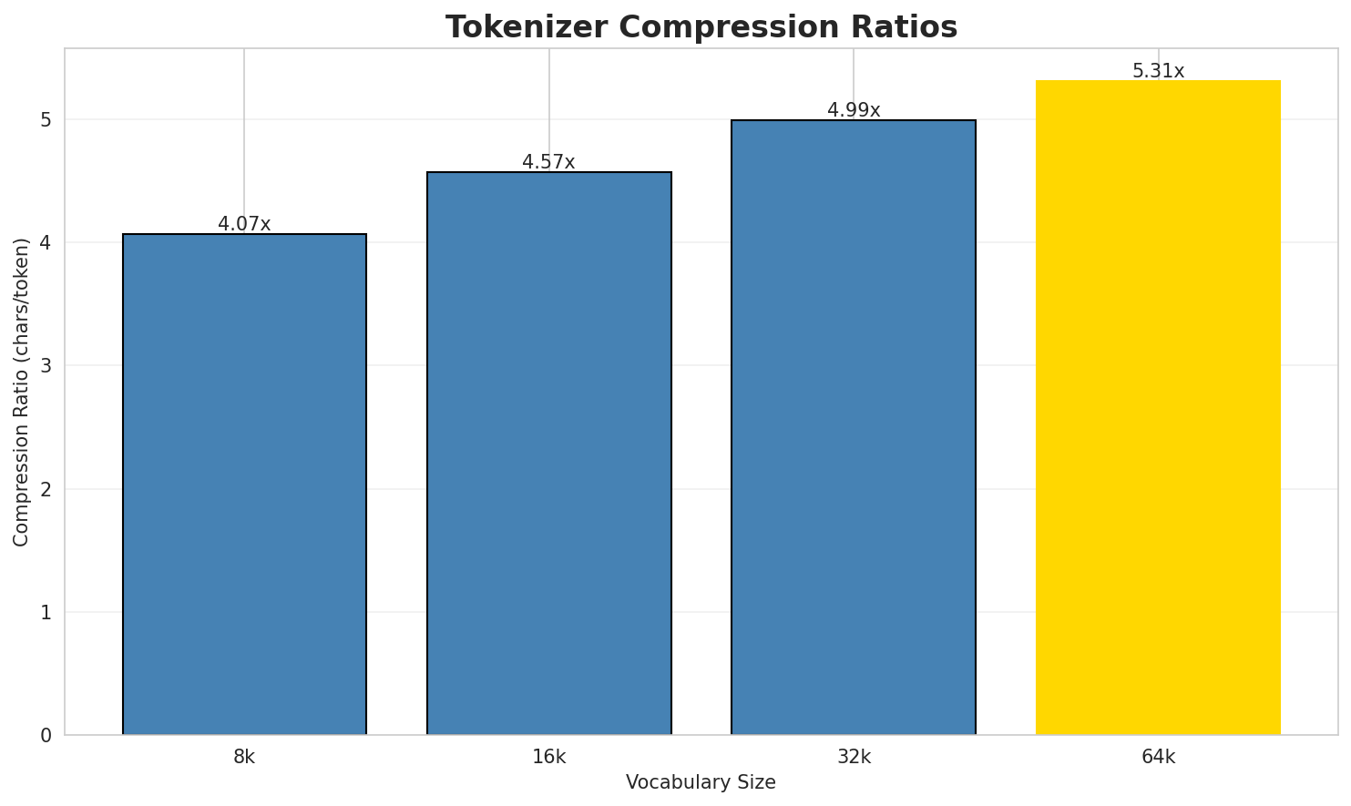
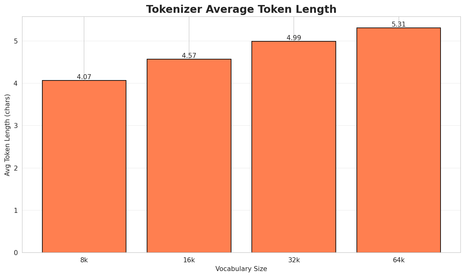
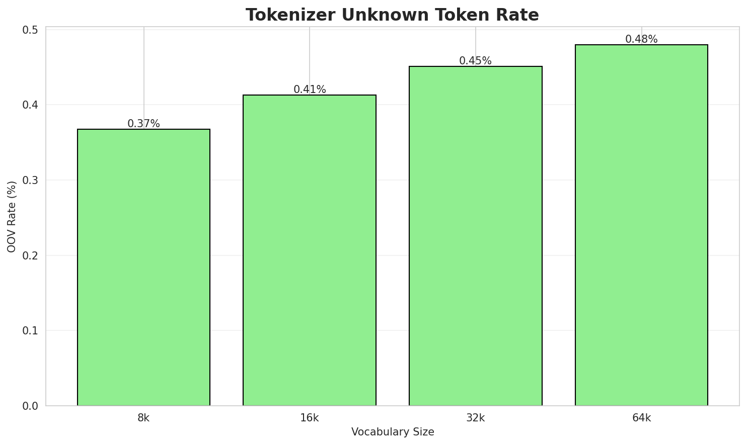
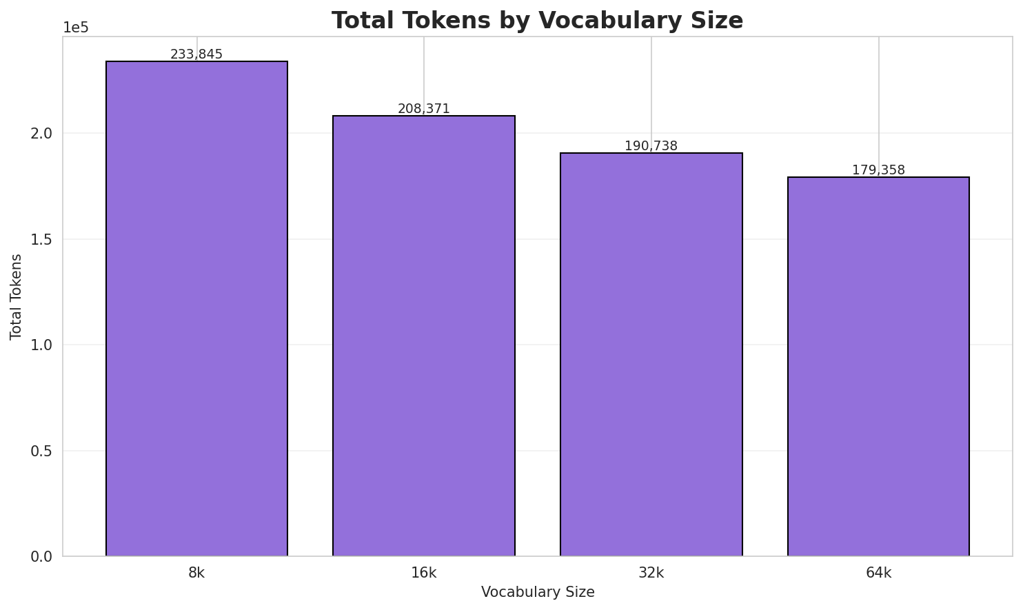
| Vocab Size | Compression | Avg Token Len | UNK Rate | Total Tokens |
|---|---|---|---|---|
| 8k | 4.069x | 4.07 | 0.3678% | 233,845 |
| 16k | 4.567x | 4.57 | 0.4127% | 208,371 |
| 32k | 4.989x | 4.99 | 0.4509% | 190,738 |
| 64k | 5.306x 🏆 | 5.31 | 0.4795% | 179,358 |
Tokenization Examples
Below are sample sentences tokenized with each vocabulary size:
Sample 1: གསེར་མོ་ནི་སྒོང་སྐྱེས་སྲོག་ཆགས་ཀྱི་རིགས་གཅིག་རེད། ལོ་རྒྱུས། པར་རིས་བར་འཁྱམས། ཟིན...
| Vocab | Tokens | Count |
|---|---|---|
| 8k | ▁གསེར་ མོ་ནི་ སྒོང་སྐྱེས་ སྲོག་ཆགས་ཀྱི་ རིགས་གཅིག་རེད། ▁ལོ་རྒྱུས། ▁པར་རིས་བར་ འཁྱམས། ▁ཟིན་ཐོ་ འམ་དཔྱད་གཞི། ... (+5 more) |
15 |
| 16k | ▁གསེར་ མོ་ནི་ སྒོང་སྐྱེས་ སྲོག་ཆགས་ཀྱི་ རིགས་གཅིག་རེད། ▁ལོ་རྒྱུས། ▁པར་རིས་བར་ འཁྱམས། ▁ཟིན་ཐོ་ འམ་དཔྱད་གཞི། ... (+5 more) |
15 |
| 32k | ▁གསེར་ མོ་ནི་ སྒོང་སྐྱེས་ སྲོག་ཆགས་ཀྱི་ རིགས་གཅིག་རེད། ▁ལོ་རྒྱུས། ▁པར་རིས་བར་ འཁྱམས། ▁ཟིན་ཐོ་ འམ་དཔྱད་གཞི། ... (+5 more) |
15 |
| 64k | ▁གསེར་ མོ་ནི་ སྒོང་སྐྱེས་ སྲོག་ཆགས་ཀྱི་ རིགས་གཅིག་རེད། ▁ལོ་རྒྱུས། ▁པར་རིས་བར་ འཁྱམས། ▁ཟིན་ཐོ་ འམ་དཔྱད་གཞི། ... (+5 more) |
15 |
Sample 2: ཀྲོའུ་སི། ཞི་ལའི་ལྷ་སྒྲུང་ཁྲོད་ཀྱི་ལྷ་རེད། མི་ཚེ། པར་རིས་བར་འཁྱམས། ཟིན་ཐོ་འམ་དཔྱ...
| Vocab | Tokens | Count |
|---|---|---|
| 8k | ▁ཀྲ ོའུ་ སི། ▁ཞི་ ལའི་ ལྷ་ སྒྲུང་ ཁྲོད་ཀྱི་ ལྷ་ རེད། ... (+10 more) |
20 |
| 16k | ▁ཀྲོའུ་ སི། ▁ཞི་ ལའི་ ལྷ་སྒྲུང་ ཁྲོད་ཀྱི་ ལྷ་རེད། ▁མི་ཚེ། ▁པར་རིས་བར་ འཁྱམས། ... (+7 more) |
17 |
| 32k | ▁ཀྲོའུ་ སི། ▁ཞི་ ལའི་ ལྷ་སྒྲུང་ ཁྲོད་ཀྱི་ ལྷ་རེད། ▁མི་ཚེ། ▁པར་རིས་བར་ འཁྱམས། ... (+7 more) |
17 |
| 64k | ▁ཀྲོའུ་ སི། ▁ཞི་ ལའི་ ལྷ་སྒྲུང་ ཁྲོད་ཀྱི་ ལྷ་རེད། ▁མི་ཚེ། ▁པར་རིས་བར་ འཁྱམས། ... (+7 more) |
17 |
Sample 3: མྱང་འདས་གཞན་ནས་སྒྲུབ་ཏུ་མེད། མྱ་ངན་ལས་འདས་པ་སྟེ་ཐར་པ་དང་། ཐམས་ཅད་མཁྱེན་པའི་གོ་འཕ...
| Vocab | Tokens | Count |
|---|---|---|
| 8k | ▁མྱང་ འདས་ གཞན་ ནས་ སྒྲུབ་ ཏུ་ མེད། ▁མྱ་ངན་ ལས་འདས་ པ་སྟེ་ ... (+15 more) |
25 |
| 16k | ▁མྱང་འདས་ གཞན་ ནས་ སྒྲུབ་ ཏུ་ མེད། ▁མྱ་ངན་ ལས་འདས་ པ་སྟེ་ ཐར་ ... (+13 more) |
23 |
| 32k | ▁མྱང་འདས་ གཞན་ནས་ སྒྲུབ་ ཏུ་ མེད། ▁མྱ་ངན་ ལས་འདས་ པ་སྟེ་ ཐར་ པ་དང་། ... (+10 more) |
20 |
| 64k | ▁མྱང་འདས་ གཞན་ནས་ སྒྲུབ་ ཏུ་ མེད། ▁མྱ་ངན་ལས་འདས་ པ་སྟེ་ ཐར་ པ་དང་། ▁ཐམས་ཅད་ ... (+7 more) |
17 |
Key Findings
- Best Compression: 64k achieves 5.306x compression
- Lowest UNK Rate: 8k with 0.3678% unknown tokens
- Trade-off: Larger vocabularies improve compression but increase model size
- Recommendation: 32k vocabulary provides optimal balance for production use
2. N-gram Model Evaluation
Results
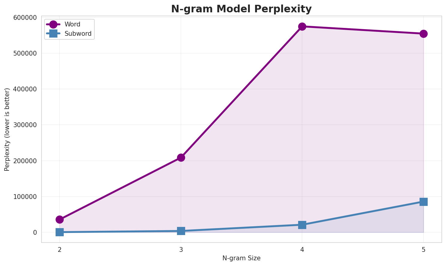
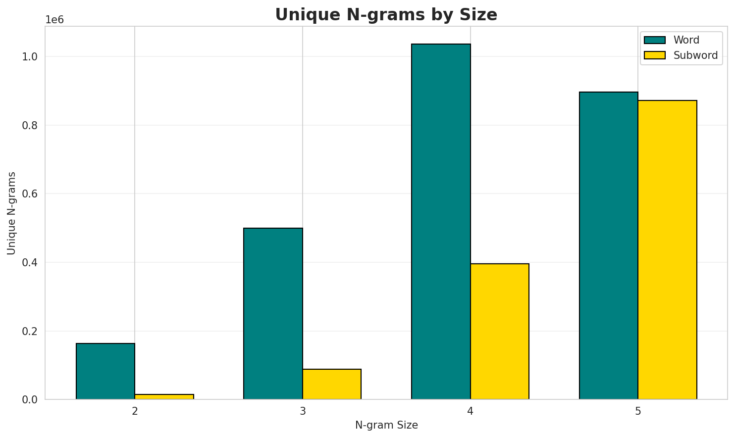
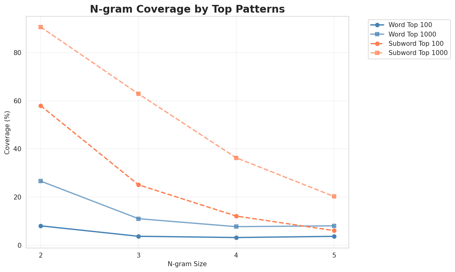
| N-gram | Variant | Perplexity | Entropy | Unique N-grams | Top-100 Coverage | Top-1000 Coverage |
|---|---|---|---|---|---|---|
| 2-gram | Word | 35,575 | 15.12 | 163,426 | 8.0% | 26.6% |
| 2-gram | Subword | 468 🏆 | 8.87 | 14,902 | 58.0% | 90.7% |
| 3-gram | Word | 208,497 | 17.67 | 499,603 | 3.7% | 11.0% |
| 3-gram | Subword | 3,697 | 11.85 | 87,521 | 25.1% | 62.9% |
| 4-gram | Word | 574,996 | 19.13 | 1,035,818 | 3.2% | 7.7% |
| 4-gram | Subword | 21,129 | 14.37 | 395,961 | 12.1% | 36.3% |
| 5-gram | Word | 554,814 | 19.08 | 896,814 | 3.6% | 8.0% |
| 5-gram | Subword | 85,765 | 16.39 | 872,546 | 6.0% | 20.2% |
Top 5 N-grams by Size
2-grams (Word):
| Rank | N-gram | Count |
|---|---|---|
| 1 | པ དང |
28,306 |
| 2 | བ དང |
12,858 |
| 3 | པ ལ |
12,495 |
| 4 | ཐམས ཅད |
12,121 |
| 5 | པ ནི |
11,602 |
3-grams (Word):
| Rank | N-gram | Count |
|---|---|---|
| 1 | སྤྱོད འཇུག གི |
4,094 |
| 2 | ཞེས བྱ བ |
3,742 |
| 3 | ད དུང གཟིགས |
3,594 |
| 4 | ཕྱོགས དྲ མཐུད |
3,563 |
| 5 | ཕྱི ཕྱོགས དྲ |
3,563 |
4-grams (Word):
| Rank | N-gram | Count |
|---|---|---|
| 1 | ཕྱི ཕྱོགས དྲ མཐུད |
3,562 |
| 2 | དཔྱད གཞིའི དཀར ཆག |
3,391 |
| 3 | ཟིན ཐོ འམ དཔྱད |
2,805 |
| 4 | ཐོ འམ དཔྱད གཞི |
2,802 |
| 5 | དུང གཟིགས ཕྱི ཕྱོགས |
2,789 |
5-grams (Word):
| Rank | N-gram | Count |
|---|---|---|
| 1 | ཟིན ཐོ འམ དཔྱད གཞི |
2,802 |
| 2 | ད དུང གཟིགས ཕྱི ཕྱོགས |
2,789 |
| 3 | གཟིགས ཕྱི ཕྱོགས དྲ མཐུད |
2,779 |
| 4 | དཀར ཆག ད དུང གཟིགས |
2,777 |
| 5 | དཔྱད གཞིའི དཀར ཆག ད |
2,776 |
2-grams (Subword):
| Rank | N-gram | Count |
|---|---|---|
| 1 | ས ་ |
1,109,782 |
| 2 | ། _ |
814,181 |
| 3 | ང ་ |
726,970 |
| 4 | ན ་ |
605,125 |
| 5 | ་ བ |
601,943 |
3-grams (Subword):
| Rank | N-gram | Count |
|---|---|---|
| 1 | ་ པ ་ |
233,799 |
| 2 | ག ས ་ |
214,635 |
| 3 | ། _ ། |
181,451 |
| 4 | ས ་ པ |
169,152 |
| 5 | ་ ད ང |
160,512 |
4-grams (Subword):
| Rank | N-gram | Count |
|---|---|---|
| 1 | ་ ད ང ་ |
137,863 |
| 2 | ་ པ འི ་ |
114,983 |
| 3 | ང ་ ། _ |
88,853 |
| 4 | ས ་ པ ་ |
77,821 |
| 5 | ་ པ ར ་ |
67,023 |
5-grams (Subword):
| Rank | N-gram | Count |
|---|---|---|
| 1 | ད ང ་ ། _ |
50,908 |
| 2 | ་ ད ང ་ ། |
50,893 |
| 3 | ས ་ པ འི ་ |
39,175 |
| 4 | ་ རྣ མ ས ་ |
29,571 |
| 5 | ་ སོ ག ས ་ |
28,140 |
Key Findings
- Best Perplexity: 2-gram (subword) with 468
- Entropy Trend: Decreases with larger n-grams (more predictable)
- Coverage: Top-1000 patterns cover ~20% of corpus
- Recommendation: 4-gram or 5-gram for best predictive performance
3. Markov Chain Evaluation
Results
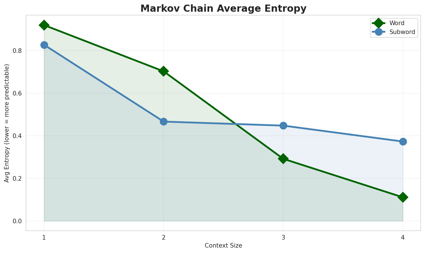
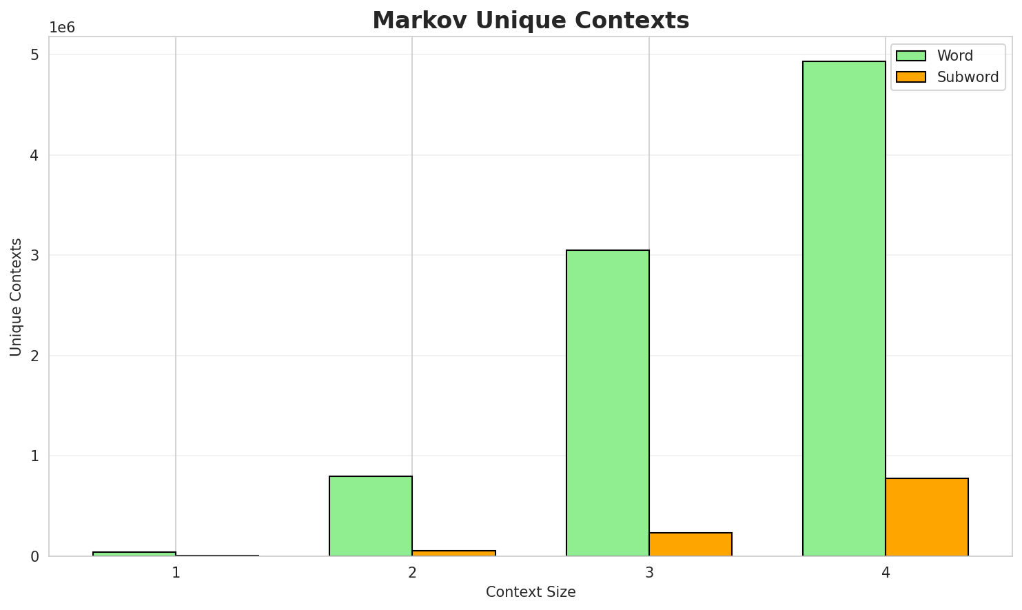
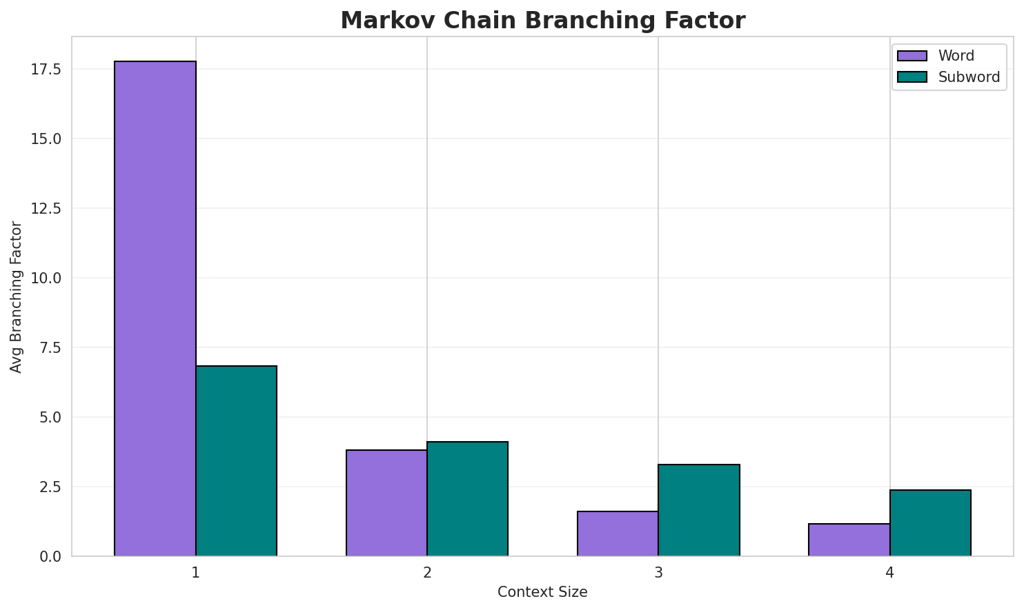
| Context | Variant | Avg Entropy | Perplexity | Branching Factor | Unique Contexts | Predictability |
|---|---|---|---|---|---|---|
| 1 | Word | 0.9206 | 1.893 | 17.76 | 45,103 | 7.9% |
| 1 | Subword | 0.8281 | 1.775 | 6.83 | 8,393 | 17.2% |
| 2 | Word | 0.7033 | 1.628 | 3.81 | 800,524 | 29.7% |
| 2 | Subword | 0.4670 | 1.382 | 4.11 | 57,328 | 53.3% |
| 3 | Word | 0.2921 | 1.224 | 1.62 | 3,051,550 | 70.8% |
| 3 | Subword | 0.4481 | 1.364 | 3.28 | 235,662 | 55.2% |
| 4 | Word | 0.1112 🏆 | 1.080 | 1.18 | 4,929,019 | 88.9% |
| 4 | Subword | 0.3733 | 1.295 | 2.38 | 773,603 | 62.7% |
Generated Text Samples (Word-based)
Below are text samples generated from each word-based Markov chain model:
Context Size 1:
པ ཡིད གཉིས གདན ཤོ མིག གསུམ རྫིང བུར ལན གསུམ པ ལ མཱུ ཥི ཏདང སུམ གཉིས ཀྱི ཞབས ལྕགས རིགས སུ བཞུགས པ ཆེན མོ གཉིས ཀྱི ཚད ལསལ བོད ཤན ནམ ཞིག ལུས ལ སོགས པའི མིང པེལ རེས མོས བརྡུང བའི སྐུ
Context Size 2:
པ དང གདམ ང མ གཉིས གཉིས གཉིས ཡོད ཤར ཕོགས ཀི པཎི ཏ ཨ བྷི ཥིཉྩབ དང མནའ སྐྱེལ ཞིང དབྱར ཀ རི ཀ སྤྱི མཐུན རྒྱལ ཁབ དེ རུ བཞག གོཔ ལ བཞུགས པར ཞལ གྱིས བཞེས པ ནས འབྲས བུ ཉེ ཟ དེའི བྱེ བྲག པ
Context Size 3:
སྤྱོད འཇུག གི དཀའ འགྲེལ ཤིང དཔར ཞེས གསུངས པ ནི འདོད པ ཁྱབ ཁོངས ཡངས པ དེཞེས བྱ བ ལ སོགས པ གཞན མ ཡིན ནོ རབ འབར དགྲ ཡི དབང དུ ཟད འཕེལད དུང གཟིགས ཕྱི ཕྱོགས དྲ མཐུད ལྕེ དཔྱད གཞིའི དཀར ཆག ད དུང གཟིགས ཀྱེ རྡོ རྗེ
Context Size 4:
དཔྱད གཞིའི དཀར ཆག ད དུང གཟིགས ཕྱི ཕྱོགས དྲ མཐུད དབྱིན ཇིའི རླུང འཕྲིན ཀུང སིས ཉིན དེརཟིན ཐོ འམ དཔྱད གཞི དཔྱད གཞིའི དཀར ཆག ད དུང གཟིགས ཕྱི ཕྱོགས དྲ མཐུད bdrc buddhist digitalཐོ འམ དཔྱད གཞི དཔྱད གཞིའི དཀར ཆག ད དུང གཟིགས གེ སར རྒྱལ པོ རྒྱ ནག ཏུ ཕེབས
Generated Text Samples (Subword-based)
Below are text samples generated from each subword-based Markov chain model:
Context Size 1:
་དུ་མོ་སྦྱངས་མསལ་ཁྲི་ཁས་ཉིས།_ཞནང་ཀྱིས།_དངགས་ཆེན་ནི་ཡོད་འ༔_།_
Context Size 2:
ས་དངོས་ཀྱི་ལྷས་ད་ེ_རྣམས།_ཁེངས་བཞིན་པའི་སྡུག་ཡིང་།_ད་གཉིས།_དྲངས་པར
Context Size 3:
་པ་ལ་དྲིས་ན་ནི་_ལོའི་རྒྱུདགས་པ་གླིང་བཙན་པོ་དབྱིངས།_།བྱས་ཀྱང་རུང་།_མི་དང
Context Size 4:
་དང་།_།མཐུ་སྟོབས་རྒྱས་མཛེ་པའི་ཚུལ་བཻ་སེར་པོ་འཁོར་ཡང་།_བཞི་པ།_སྟོན་པ་སྒྲུབ་པ
Key Findings
- Best Predictability: Context-4 (word) with 88.9% predictability
- Branching Factor: Decreases with context size (more deterministic)
- Memory Trade-off: Larger contexts require more storage (773,603 contexts)
- Recommendation: Context-3 or Context-4 for text generation
4. Vocabulary Analysis
Statistics
| Metric | Value |
|---|---|
| Vocabulary Size | 18,977 |
| Total Tokens | 7,591,805 |
| Mean Frequency | 400.05 |
| Median Frequency | 5 |
| Frequency Std Dev | 3886.00 |
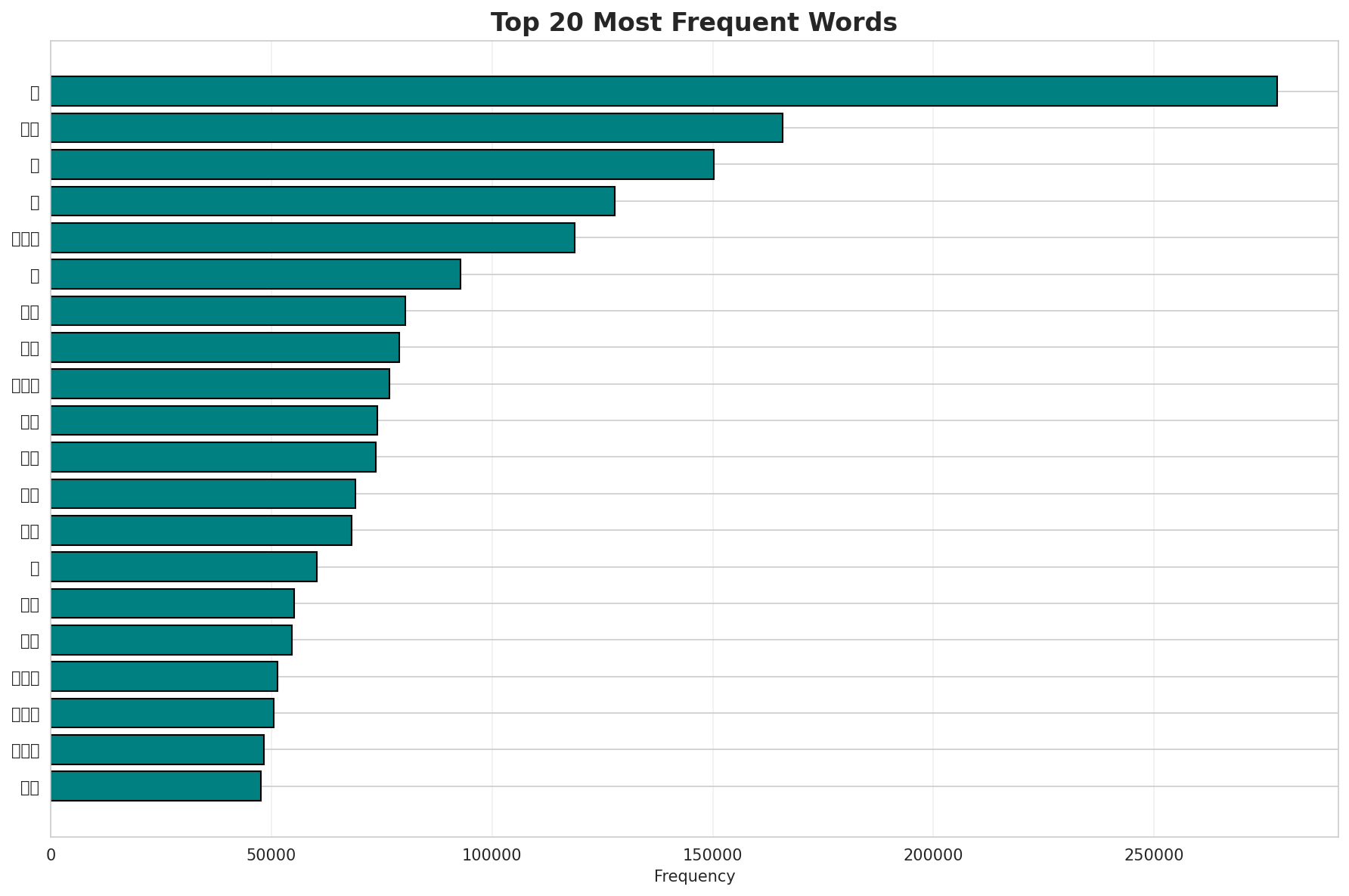
Most Common Words
| Rank | Word | Frequency |
|---|---|---|
| 1 | པ | 277,831 |
| 2 | དང | 165,810 |
| 3 | ལ | 150,300 |
| 4 | བ | 127,823 |
| 5 | པའི | 118,705 |
| 6 | མ | 92,873 |
| 7 | དེ | 80,387 |
| 8 | ནི | 78,884 |
| 9 | ཀྱི | 76,665 |
| 10 | དུ | 73,981 |
Least Common Words (from vocabulary)
| Rank | Word | Frequency |
|---|---|---|
| 1 | སུམྦྷའི | 2 |
| 2 | བིཀྲ | 2 |
| 3 | jayasena | 2 |
| 4 | ཤུདྡྷཿསརྦྦ | 2 |
| 5 | ཧྲོཾ | 2 |
| 6 | ཝརྞཱ | 2 |
| 7 | caryā | 2 |
| 8 | gīti | 2 |
| 9 | caryāgītivṛtti | 2 |
| 10 | དཀྲྀཏ | 2 |
Zipf's Law Analysis
| Metric | Value |
|---|---|
| Zipf Coefficient | 2.0091 |
| R² (Goodness of Fit) | 0.961368 |
| Adherence Quality | excellent |
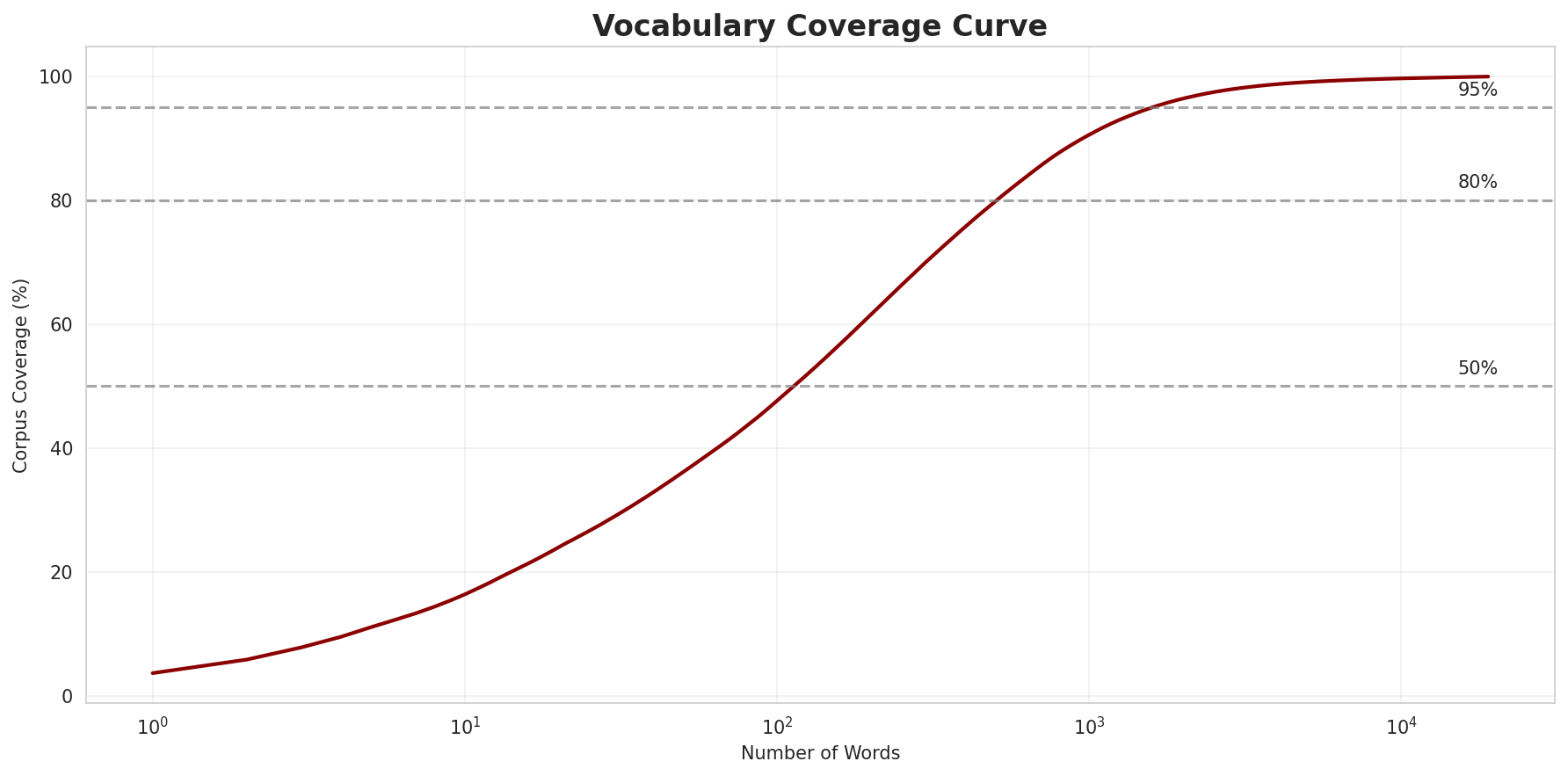
Coverage Analysis
| Top N Words | Coverage |
|---|---|
| Top 100 | 47.6% |
| Top 1,000 | 90.6% |
| Top 5,000 | 99.1% |
| Top 10,000 | 99.7% |
Key Findings
- Zipf Compliance: R²=0.9614 indicates excellent adherence to Zipf's law
- High Frequency Dominance: Top 100 words cover 47.6% of corpus
- Long Tail: 8,977 words needed for remaining 0.3% coverage
5. Word Embeddings Evaluation
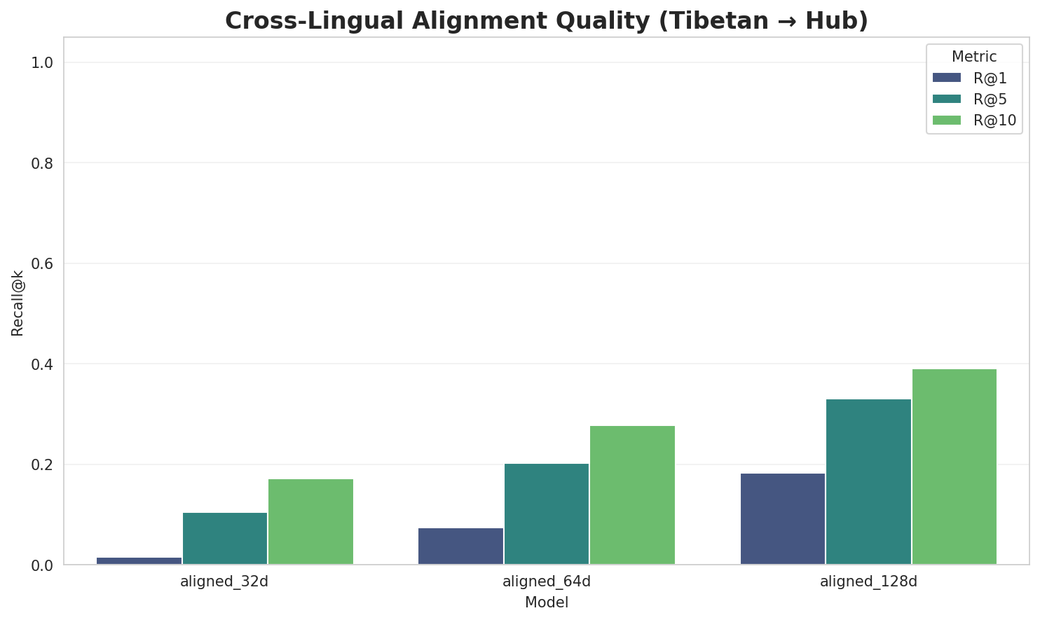
5.1 Cross-Lingual Alignment
5.2 Model Comparison
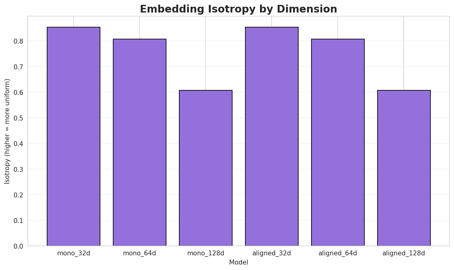
| Model | Dimension | Isotropy | Semantic Density | Alignment R@1 | Alignment R@10 |
|---|---|---|---|---|---|
| mono_32d | 32 | 0.8542 🏆 | 0.3709 | N/A | N/A |
| mono_64d | 64 | 0.8068 | 0.3078 | N/A | N/A |
| mono_128d | 128 | 0.6072 | 0.2915 | N/A | N/A |
| aligned_32d | 32 | 0.8542 | 0.3660 | 0.0160 | 0.1720 |
| aligned_64d | 64 | 0.8068 | 0.3152 | 0.0740 | 0.2780 |
| aligned_128d | 128 | 0.6072 | 0.2869 | 0.1820 | 0.3900 |
Key Findings
- Best Isotropy: mono_32d with 0.8542 (more uniform distribution)
- Semantic Density: Average pairwise similarity of 0.3231. Lower values indicate better semantic separation.
- Alignment Quality: Aligned models achieve up to 18.2% R@1 in cross-lingual retrieval.
- Recommendation: 128d aligned for best cross-lingual performance
6. Morphological Analysis (Experimental)
This section presents an automated morphological analysis derived from the statistical divergence between word-level and subword-level models. By analyzing where subword predictability spikes and where word-level coverage fails, we can infer linguistic structures without supervised data.
6.1 Productivity & Complexity
| Metric | Value | Interpretation | Recommendation |
|---|---|---|---|
| Productivity Index | 5.000 | High morphological productivity | Reliable analysis |
| Idiomaticity Gap | -0.603 | Low formulaic content | - |
6.2 Affix Inventory (Productive Units)
These are the most productive prefixes and suffixes identified by sampling the vocabulary for global substitutability patterns. A unit is considered an affix if stripping it leaves a valid stem that appears in other contexts.
No productive affixes detected.
6.3 Bound Stems (Lexical Roots)
Bound stems are high-frequency subword units that are semantically cohesive but rarely appear as standalone words. These often correspond to the 'core' of a word that requires inflection or derivation to be valid.
No significant bound stems detected.
6.4 Affix Compatibility (Co-occurrence)
This table shows which prefixes and suffixes most frequently co-occur on the same stems, revealing the 'stacking' rules of the language's morphology.
No significant affix co-occurrences detected.
6.5 Recursive Morpheme Segmentation
Using Recursive Hierarchical Substitutability, we decompose complex words into their constituent morphemes. This approach handles nested affixes (e.g., prefix-prefix-root-suffix).
Insufficient data for recursive segmentation.
6.6 Linguistic Interpretation
Automated Insight: The language Tibetan shows high morphological productivity. The subword models are significantly more efficient than word models, suggesting a rich system of affixation or compounding.
7. Summary & Recommendations
Production Recommendations
| Component | Recommended | Rationale |
|---|---|---|
| Tokenizer | 64k BPE | Best compression (5.31x) |
| N-gram | 2-gram | Lowest perplexity (468) |
| Markov | Context-4 | Highest predictability (88.9%) |
| Embeddings | 100d | Balanced semantic capture and isotropy |
Appendix: Metrics Glossary & Interpretation Guide
This section provides definitions, intuitions, and guidance for interpreting the metrics used throughout this report.
Tokenizer Metrics
Compression Ratio
Definition: The ratio of characters to tokens (chars/token). Measures how efficiently the tokenizer represents text.
Intuition: Higher compression means fewer tokens needed to represent the same text, reducing sequence lengths for downstream models. A 3x compression means ~3 characters per token on average.
What to seek: Higher is generally better for efficiency, but extremely high compression may indicate overly aggressive merging that loses morphological information.
Average Token Length (Fertility)
Definition: Mean number of characters per token produced by the tokenizer.
Intuition: Reflects the granularity of tokenization. Longer tokens capture more context but may struggle with rare words; shorter tokens are more flexible but increase sequence length.
What to seek: Balance between 2-5 characters for most languages. Arabic/morphologically-rich languages may benefit from slightly longer tokens.
Unknown Token Rate (OOV Rate)
Definition: Percentage of tokens that map to the unknown/UNK token, indicating words the tokenizer cannot represent.
Intuition: Lower OOV means better vocabulary coverage. High OOV indicates the tokenizer encounters many unseen character sequences.
What to seek: Below 1% is excellent; below 5% is acceptable. BPE tokenizers typically achieve very low OOV due to subword fallback.
N-gram Model Metrics
Perplexity
Definition: Measures how "surprised" the model is by test data. Mathematically: 2^(cross-entropy). Lower values indicate better prediction.
Intuition: If perplexity is 100, the model is as uncertain as if choosing uniformly among 100 options at each step. A perplexity of 10 means effectively choosing among 10 equally likely options.
What to seek: Lower is better. Perplexity decreases with larger n-grams (more context). Values vary widely by language and corpus size.
Entropy
Definition: Average information content (in bits) needed to encode the next token given the context. Related to perplexity: perplexity = 2^entropy.
Intuition: High entropy means high uncertainty/randomness; low entropy means predictable patterns. Natural language typically has entropy between 1-4 bits per character.
What to seek: Lower entropy indicates more predictable text patterns. Entropy should decrease as n-gram size increases.
Coverage (Top-K)
Definition: Percentage of corpus occurrences explained by the top K most frequent n-grams.
Intuition: High coverage with few patterns indicates repetitive/formulaic text; low coverage suggests diverse vocabulary usage.
What to seek: Depends on use case. For language modeling, moderate coverage (40-60% with top-1000) is typical for natural text.
Markov Chain Metrics
Average Entropy
Definition: Mean entropy across all contexts, measuring average uncertainty in next-word prediction.
Intuition: Lower entropy means the model is more confident about what comes next. Context-1 has high entropy (many possible next words); Context-4 has low entropy (few likely continuations).
What to seek: Decreasing entropy with larger context sizes. Very low entropy (<0.1) indicates highly deterministic transitions.
Branching Factor
Definition: Average number of unique next tokens observed for each context.
Intuition: High branching = many possible continuations (flexible but uncertain); low branching = few options (predictable but potentially repetitive).
What to seek: Branching factor should decrease with context size. Values near 1.0 indicate nearly deterministic chains.
Predictability
Definition: Derived metric: (1 - normalized_entropy) × 100%. Indicates how deterministic the model's predictions are.
Intuition: 100% predictability means the next word is always certain; 0% means completely random. Real text falls between these extremes.
What to seek: Higher predictability for text generation quality, but too high (>98%) may produce repetitive output.
Vocabulary & Zipf's Law Metrics
Zipf's Coefficient
Definition: The slope of the log-log plot of word frequency vs. rank. Zipf's law predicts this should be approximately -1.
Intuition: A coefficient near -1 indicates the corpus follows natural language patterns where a few words are very common and most words are rare.
What to seek: Values between -0.8 and -1.2 indicate healthy natural language distribution. Deviations may suggest domain-specific or artificial text.
R² (Coefficient of Determination)
Definition: Measures how well the linear fit explains the frequency-rank relationship. Ranges from 0 to 1.
Intuition: R² near 1.0 means the data closely follows Zipf's law; lower values indicate deviation from expected word frequency patterns.
What to seek: R² > 0.95 is excellent; > 0.99 indicates near-perfect Zipf adherence typical of large natural corpora.
Vocabulary Coverage
Definition: Cumulative percentage of corpus tokens accounted for by the top N words.
Intuition: Shows how concentrated word usage is. If top-100 words cover 50% of text, the corpus relies heavily on common words.
What to seek: Top-100 covering 30-50% is typical. Higher coverage indicates more repetitive text; lower suggests richer vocabulary.
Word Embedding Metrics
Isotropy
Definition: Measures how uniformly distributed vectors are in the embedding space. Computed as the ratio of minimum to maximum singular values.
Intuition: High isotropy (near 1.0) means vectors spread evenly in all directions; low isotropy means vectors cluster in certain directions, reducing expressiveness.
What to seek: Higher isotropy generally indicates better-quality embeddings. Values > 0.1 are reasonable; > 0.3 is good. Lower-dimensional embeddings tend to have higher isotropy.
Average Norm
Definition: Mean magnitude (L2 norm) of word vectors in the embedding space.
Intuition: Indicates the typical "length" of vectors. Consistent norms suggest stable training; high variance may indicate some words are undertrained.
What to seek: Relatively consistent norms across models. The absolute value matters less than consistency (low std deviation).
Cosine Similarity
Definition: Measures angular similarity between vectors, ranging from -1 (opposite) to 1 (identical direction).
Intuition: Words with similar meanings should have high cosine similarity. This is the standard metric for semantic relatedness in embeddings.
What to seek: Semantically related words should score > 0.5; unrelated words should be near 0. Synonyms often score > 0.7.
t-SNE Visualization
Definition: t-Distributed Stochastic Neighbor Embedding - a dimensionality reduction technique that preserves local structure for visualization.
Intuition: Clusters in t-SNE plots indicate groups of semantically related words. Spread indicates vocabulary diversity; tight clusters suggest semantic coherence.
What to seek: Meaningful clusters (e.g., numbers together, verbs together). Avoid over-interpreting distances - t-SNE preserves local, not global, structure.
General Interpretation Guidelines
- Compare within model families: Metrics are most meaningful when comparing models of the same type (e.g., 8k vs 64k tokenizer).
- Consider trade-offs: Better performance on one metric often comes at the cost of another (e.g., compression vs. OOV rate).
- Context matters: Optimal values depend on downstream tasks. Text generation may prioritize different metrics than classification.
- Corpus influence: All metrics are influenced by corpus characteristics. Wikipedia text differs from social media or literature.
- Language-specific patterns: Morphologically rich languages (like Arabic) may show different optimal ranges than analytic languages.
Visualizations Index
| Visualization | Description |
|---|---|
| Tokenizer Compression | Compression ratios by vocabulary size |
| Tokenizer Fertility | Average token length by vocabulary |
| Tokenizer OOV | Unknown token rates |
| Tokenizer Total Tokens | Total tokens by vocabulary |
| N-gram Perplexity | Perplexity by n-gram size |
| N-gram Entropy | Entropy by n-gram size |
| N-gram Coverage | Top pattern coverage |
| N-gram Unique | Unique n-gram counts |
| Markov Entropy | Entropy by context size |
| Markov Branching | Branching factor by context |
| Markov Contexts | Unique context counts |
| Zipf's Law | Frequency-rank distribution with fit |
| Vocab Frequency | Word frequency distribution |
| Top 20 Words | Most frequent words |
| Vocab Coverage | Cumulative coverage curve |
| Embedding Isotropy | Vector space uniformity |
| Embedding Norms | Vector magnitude distribution |
| Embedding Similarity | Word similarity heatmap |
| Nearest Neighbors | Similar words for key terms |
| t-SNE Words | 2D word embedding visualization |
| t-SNE Sentences | 2D sentence embedding visualization |
| Position Encoding | Encoding method comparison |
| Model Sizes | Storage requirements |
| Performance Dashboard | Comprehensive performance overview |
About This Project
Data Source
Models trained on wikipedia-monthly - a monthly snapshot of Wikipedia articles across 300+ languages.
Project
A project by Wikilangs - Open-source NLP models for every Wikipedia language.
Maintainer
Citation
If you use these models in your research, please cite:
@misc{wikilangs2025,
  author = {Kamali, Omar},
  title = {Wikilangs: Open NLP Models for Wikipedia Languages},
  year = {2025},
  doi = {10.5281/zenodo.18073153},
  publisher = {Zenodo},
  url = {https://huggingface.co/wikilangs}
  institution = {Omneity Labs}
}
License
MIT License - Free for academic and commercial use.
Links
- 🌐 Website: wikilangs.org
- 🤗 Models: huggingface.co/wikilangs
- 📊 Data: wikipedia-monthly
- 👤 Author: Omar Kamali
- 🤝 Sponsor: Featherless AI
Generated by Wikilangs Models Pipeline
Report Date: 2026-01-03 19:39:42

