wikilangs/mi

Māori - Wikilangs Models

Comprehensive Research Report & Full Ablation Study

This repository contains NLP models trained and evaluated by Wikilangs, specifically on Māori Wikipedia data. We analyze tokenizers, n-gram models, Markov chains, vocabulary statistics, and word embeddings.

📋 Repository Contents

Models & Assets

• Tokenizers (8k, 16k, 32k, 64k)
• N-gram models (2, 3, 4, 5-gram)
• Markov chains (context of 1, 2, 3, 4 and 5)
• Subword N-gram and Markov chains
• Embeddings in various sizes and dimensions (aligned and unaligned)
• Language Vocabulary
• Language Statistics

Analysis and Evaluation

• 1. Tokenizer Evaluation
• 2. N-gram Model Evaluation
• 3. Markov Chain Evaluation
• 4. Vocabulary Analysis
• 5. Word Embeddings Evaluation
• 6. Morphological Analysis (Experimental)
• 7. Summary & Recommendations
• Metrics Glossary
• Visualizations Index

---

1. Tokenizer Evaluation

Results

Vocab Size	Compression	Avg Token Len	UNK Rate	Total Tokens
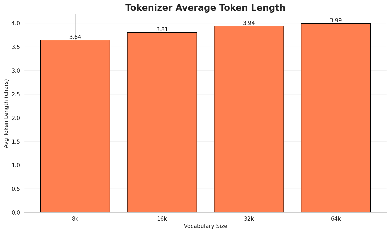
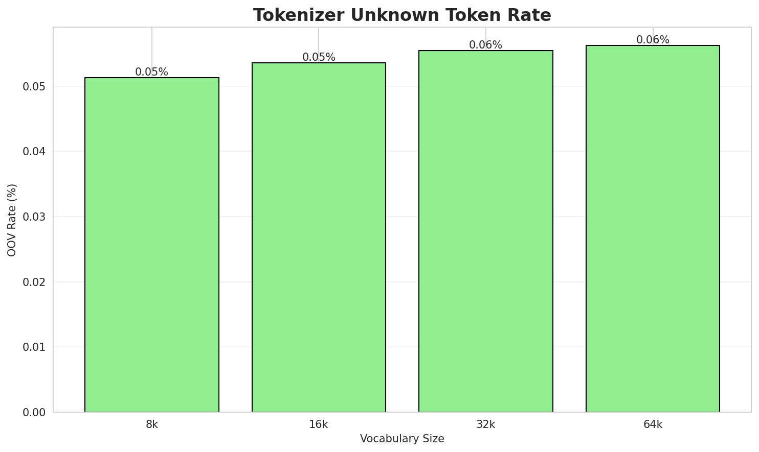
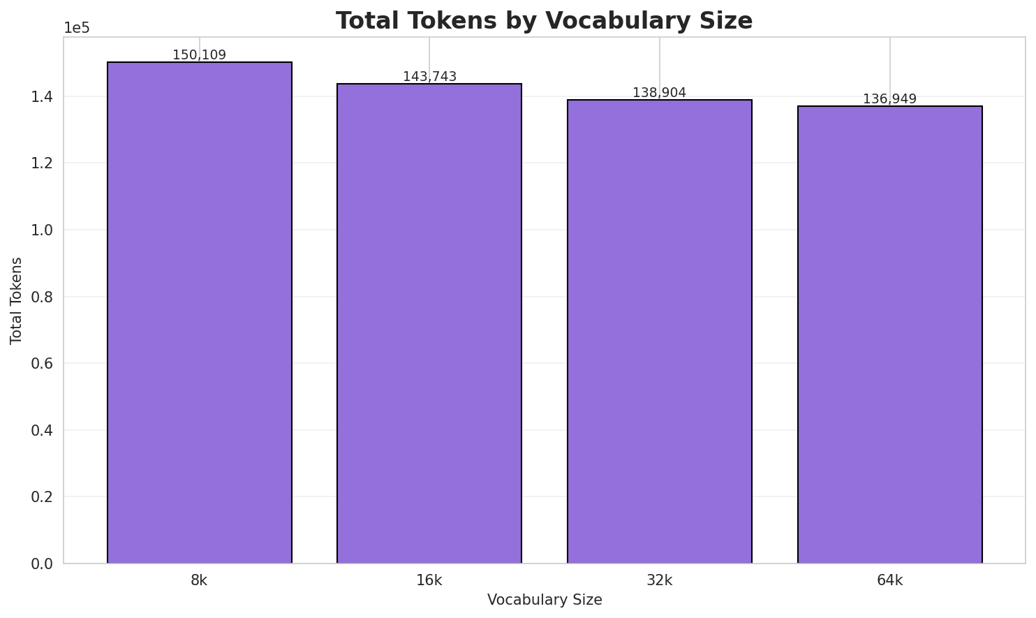
8k	3.637x	3.64	0.0513%	150,109
16k	3.798x	3.81	0.0536%	143,743
32k	3.931x	3.94	0.0554%	138,904
64k	3.987x 🏆	3.99	0.0562%	136,949

Tokenization Examples

Below are sample sentences tokenized with each vocabulary size:

Sample 1: Ko Tūnihia (reo Ārapi: الجمهورية التونسية, al-Jumhūrīyah at-Tūnisīyah) he whenua...

Vocab	Tokens	Count
8k	▁ko ▁tū nihia ▁( reo ▁ārapi : ▁ال ج م ... (+45 more)	55
16k	▁ko ▁tūnihia ▁( reo ▁ārapi : ▁ال ج مهورية ▁ال ... (+39 more)	49
32k	▁ko ▁tūnihia ▁( reo ▁ārapi : ▁الجمهورية ▁التونسية , ▁al ... (+27 more)	37
64k	▁ko ▁tūnihia ▁( reo ▁ārapi : ▁الجمهورية ▁التونسية , ▁al ... (+27 more)	37

Sample 2: Ko Kōkiri Ahitereiria Ataahua () te waiata a whenua mo Ahitereiria.

Vocab	Tokens	Count
8k	▁ko ▁kōkiri ▁ahitereiria ▁ata ahua ▁() ▁te ▁waiata ▁a ▁whenua ... (+3 more)	13
16k	▁ko ▁kōkiri ▁ahitereiria ▁ataahua ▁() ▁te ▁waiata ▁a ▁whenua ▁mo ... (+2 more)	12
32k	▁ko ▁kōkiri ▁ahitereiria ▁ataahua ▁() ▁te ▁waiata ▁a ▁whenua ▁mo ... (+2 more)	12
64k	▁ko ▁kōkiri ▁ahitereiria ▁ataahua ▁() ▁te ▁waiata ▁a ▁whenua ▁mo ... (+2 more)	12

Sample 3: Ko Kiri Te Kanawa he kaiwaiata rongonui nō Aotearoa.

Vocab	Tokens	Count
8k	▁ko ▁kiri ▁te ▁kana wa ▁he ▁kaiwaiata ▁rongonui ▁nō ▁aotearoa ... (+1 more)	11
16k	▁ko ▁kiri ▁te ▁kanawa ▁he ▁kaiwaiata ▁rongonui ▁nō ▁aotearoa .	10
32k	▁ko ▁kiri ▁te ▁kanawa ▁he ▁kaiwaiata ▁rongonui ▁nō ▁aotearoa .	10
64k	▁ko ▁kiri ▁te ▁kanawa ▁he ▁kaiwaiata ▁rongonui ▁nō ▁aotearoa .	10

Key Findings

• Best Compression: 64k achieves 3.987x compression
• Lowest UNK Rate: 8k with 0.0513% unknown tokens
• Trade-off: Larger vocabularies improve compression but increase model size
• Recommendation: 32k vocabulary provides optimal balance for production use

---

2. N-gram Model Evaluation

Results

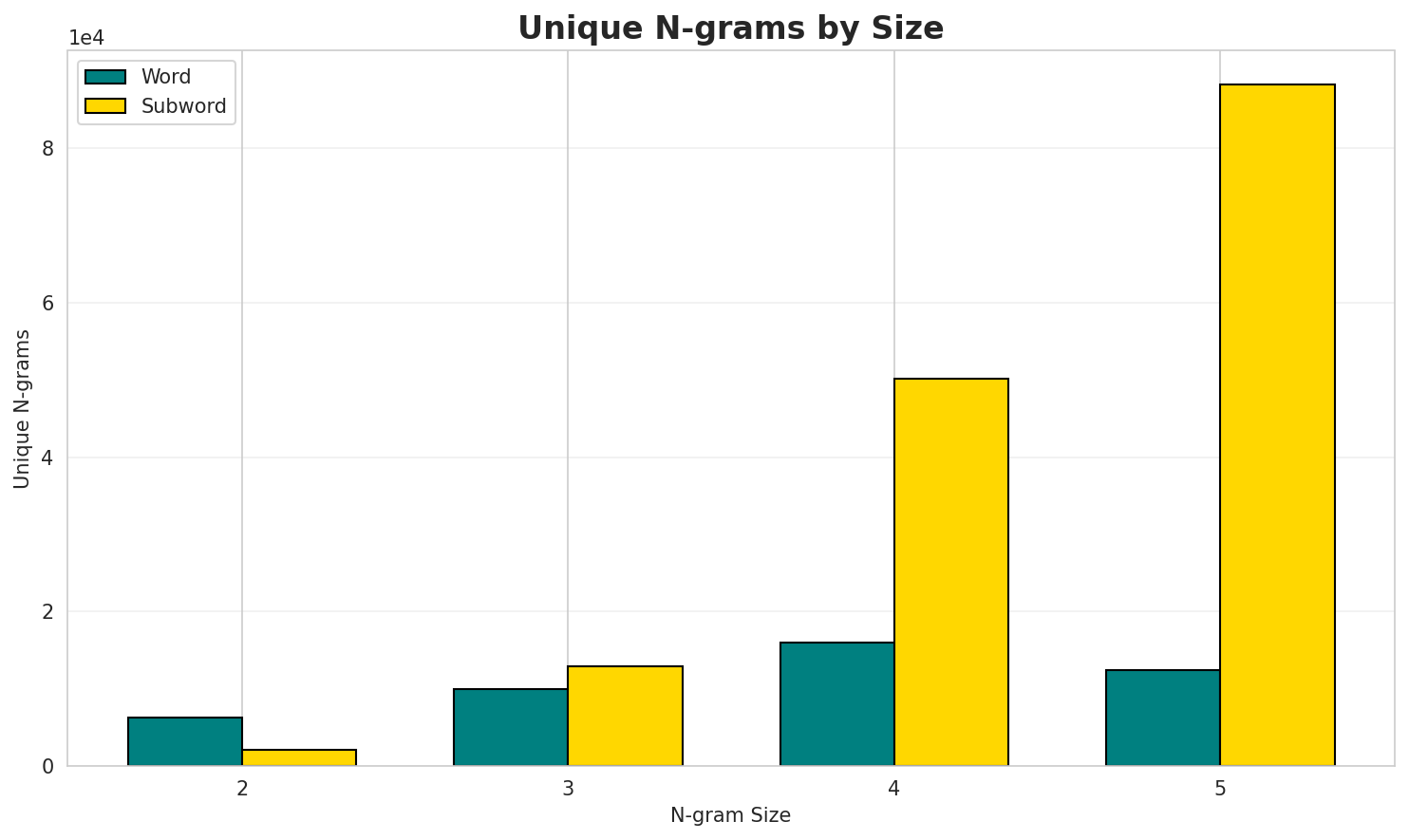
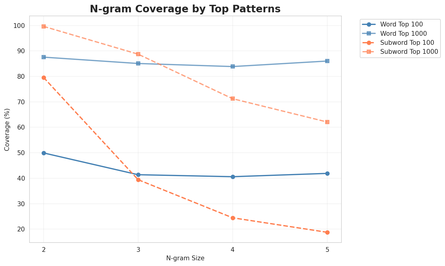
N-gram	Variant	Perplexity	Entropy	Unique N-grams	Top-100 Coverage	Top-1000 Coverage
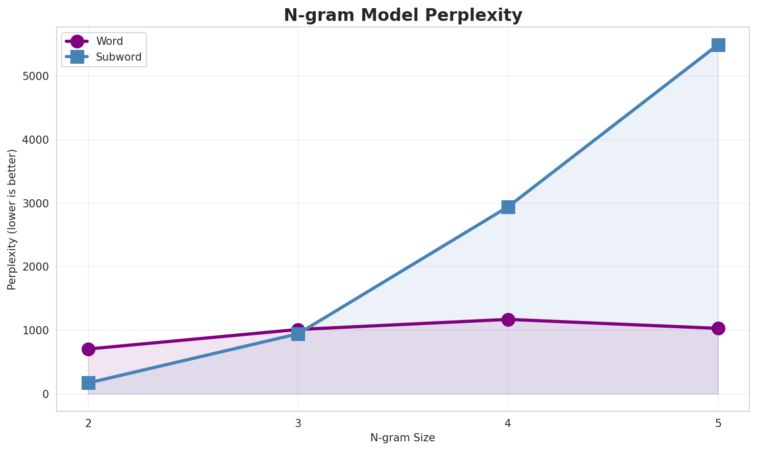
2-gram	Word	705	9.46	6,245	49.9%	87.5%
2-gram	Subword	171 🏆	7.42	2,075	79.6%	99.6%
3-gram	Word	1,013	9.98	9,926	41.4%	85.1%
3-gram	Subword	945	9.88	12,961	39.4%	88.7%
4-gram	Word	1,172	10.19	16,021	40.6%	83.8%
4-gram	Subword	2,943	11.52	50,169	24.5%	71.2%
5-gram	Word	1,030	10.01	12,463	41.9%	86.0%
5-gram	Subword	5,494	12.42	88,213	18.8%	62.1%

Top 5 N-grams by Size

2-grams (Word):

Rank	N-gram	Count
1	o te	12,376
2	ko te	7,593
3	i te	7,520
4	ki te	6,736
5	takiwā o	5,380

3-grams (Word):

Rank	N-gram	Count
1	toitū te whenua	4,800
2	kite i te	3,310
3	he mea kite	3,304
4	mea kite i	3,304
5	new zealand he	3,271

4-grams (Word):

Rank	N-gram	Count
1	mea kite i te	3,304
2	he mea kite i	3,304
3	zealand he mea kite	3,271
4	new zealand he mea	3,271
5	toitū te whenua land	3,270

5-grams (Word):

Rank	N-gram	Count
1	he mea kite i te	3,304
2	zealand he mea kite i	3,271
3	new zealand he mea kite	3,271
4	toitū te whenua land information	3,270
5	land information new zealand he	3,270

2-grams (Subword):

Rank	N-gram	Count
1	_ t	130,423
2	e _	120,072
3	i _	95,061
4	a _	80,419
5	t e	80,353

3-grams (Subword):

Rank	N-gram	Count
1	t e _	67,768
2	_ t e	62,829
3	_ o _	33,303
4	i _ t	32,362
5	e _ t	32,097

4-grams (Subword):

Rank	N-gram	Count
1	_ t e _	61,846
2	i _ t e	21,978
3	o _ t e	20,819
4	t e _ t	18,461
5	_ h e _	17,269

5-grams (Subword):

Rank	N-gram	Count
1	i _ t e _	21,833
2	o _ t e _	20,672
3	_ t e _ t	17,983
4	t e _ t a	12,754
5	_ o _ t e	12,383

Key Findings

• Best Perplexity: 2-gram (subword) with 171
• Entropy Trend: Decreases with larger n-grams (more predictable)
• Coverage: Top-1000 patterns cover ~62% of corpus
• Recommendation: 4-gram or 5-gram for best predictive performance

---

3. Markov Chain Evaluation

Results

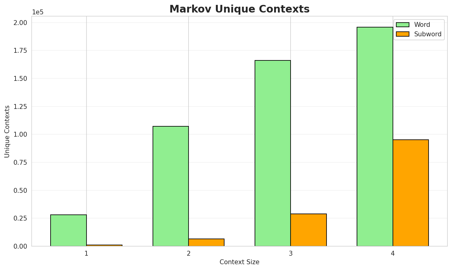
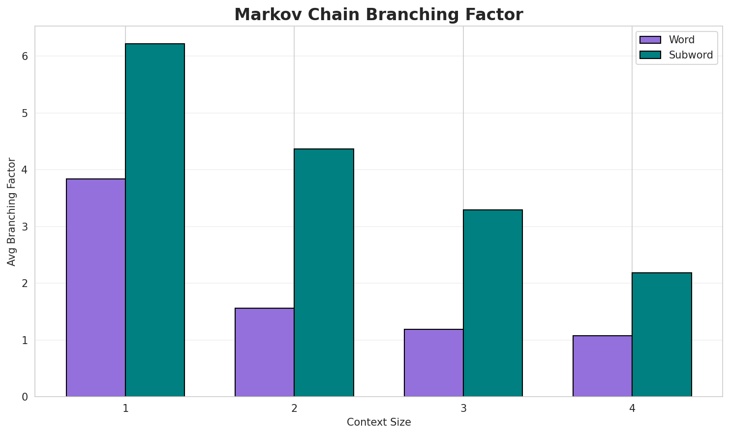
Context	Variant	Avg Entropy	Perplexity	Branching Factor	Unique Contexts	Predictability
1	Word	0.6767	1.598	3.84	28,167	32.3%
1	Subword	0.9035	1.871	6.22	1,068	9.6%
2	Word	0.2309	1.174	1.56	107,287	76.9%
2	Subword	0.7978	1.738	4.37	6,632	20.2%
3	Word	0.1002	1.072	1.19	166,148	90.0%
3	Subword	0.7225	1.650	3.30	28,939	27.7%
4	Word	0.0444 🏆	1.031	1.08	195,678	95.6%
4	Subword	0.5194	1.433	2.19	95,255	48.1%

Generated Text Samples (Word-based)

Below are text samples generated from each word-based Markov chain model:

Context Size 1:

1. te haina here turi te ope hōia ka puta ai ki toitū te kaihautū whenua he
2. o te he rite tēnei mō te takiwā ēnei whare matā pākawa pungatara s g ghost
3. ko ngā rā tonu te reo pākehā kaihautū whenua e ai ki ā nuku whiringa ā

Context Size 2:

1. o te awa garonne ko bordeaux reo wīwī bordeaux bɔʁdo reo occitan vairas te tāone nui tirohia
2. ko te he tau o te wai pounamu ko ōtepoti te tāone matua o aotearoa brainyhistory 999
3. i te reo pākehā he wāhi nohoia e te tangata engari kāore anō kia tae te nui

Context Size 3:

1. toitū te whenua he nohanga he locality rānei ki te reo pākehā he wāhi nohoia e te tangata
2. kite i te o waitaha
3. he mea kite i te o waikato en list of sgt frog characters garuru platoon ja ガルル小隊 プルル看護長

Context Size 4:

1. he mea kite i te o te moana a toi he takiwā o aotearoa kei te ika a māui
2. mea kite i te o te whanga nui a tara smith s p history and traditions of the maoris
3. new zealand he mea kite i te o te tai poutini kei te uru o te wai pounamu ko

Generated Text Samples (Subword-based)

Below are text samples generated from each subword-based Markov chain model:

Context Size 1:

1. _hanohonuhiai_tu
2. a_he_ke_i_bo_the
3. i_in_mat,_o_a_ia

Context Size 2:

1. _tionei._torahing
2. e_whi_whitū_tāorm
3. i_aotu_whe_wi_he_

Context Size 3:

1. te_paenga_o_ngā_pu
2. _te_“matahi_i_ki_a
3. _o_tāone_tāone_noh

Context Size 4:

1. _te_reo_huru_whirin
2. i_te_ai_i_te_tokera
3. o_te_papaki_te_rohe

Key Findings

• Best Predictability: Context-4 (word) with 95.6% predictability
• Branching Factor: Decreases with context size (more deterministic)
• Memory Trade-off: Larger contexts require more storage (95,255 contexts)
• Recommendation: Context-3 or Context-4 for text generation

---

4. Vocabulary Analysis

Statistics

Metric	Value
Vocabulary Size	11,670
Total Tokens	572,993
Mean Frequency	49.10
Median Frequency	3
Frequency Std Dev	801.57

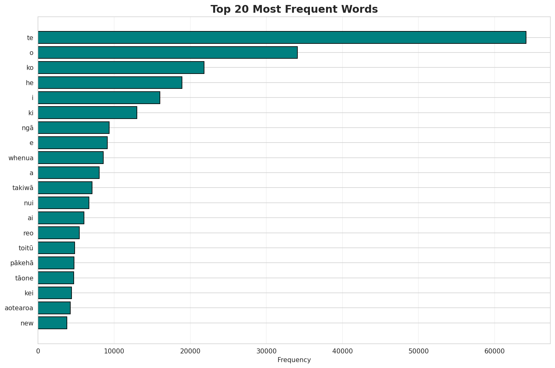
Most Common Words

Rank	Word	Frequency
1	te	64,133
2	o	34,097
3	ko	21,829
4	he	18,921
5	i	16,028
6	ki	12,979
7	ngā	9,360
8	e	9,113
9	whenua	8,565
10	a	8,027

Least Common Words (from vocabulary)

Rank	Word	Frequency
1	kaitono	2
2	dansk	2
3	ˈtænˀsk	2
4	tenemākareo	2
5	pākehāhej	2
6	fra	2
7	joāeyeshvad	2
8	hedder	2
9	lycopersicum	2
10	tomato	2

Zipf's Law Analysis

Metric	Value
Zipf Coefficient	1.2239
R² (Goodness of Fit)	0.987898
Adherence Quality	excellent

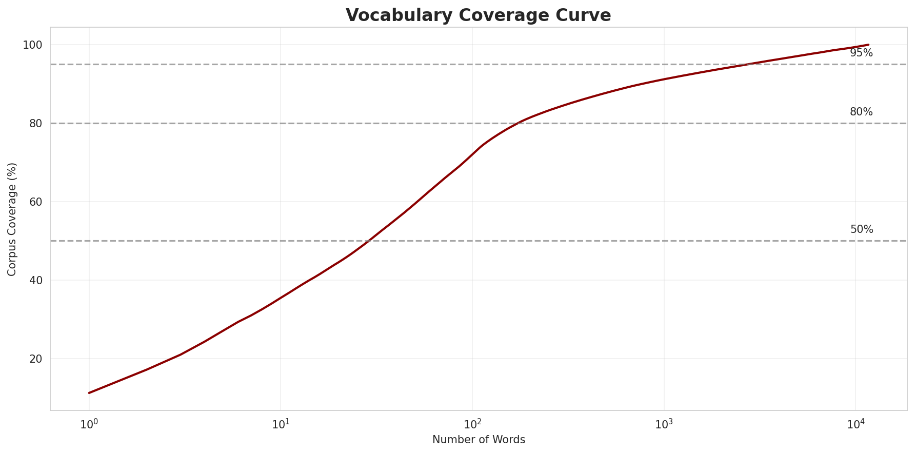
Coverage Analysis

Top N Words	Coverage
Top 100	72.0%
Top 1,000	91.2%
Top 5,000	97.1%
Top 10,000	99.4%

Key Findings

• Zipf Compliance: R²=0.9879 indicates excellent adherence to Zipf's law
• High Frequency Dominance: Top 100 words cover 72.0% of corpus
• Long Tail: 1,670 words needed for remaining 0.6% coverage

---

5. Word Embeddings Evaluation

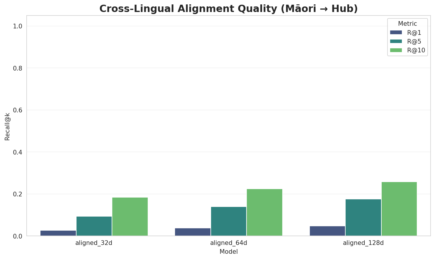
5.1 Cross-Lingual Alignment

5.2 Model Comparison

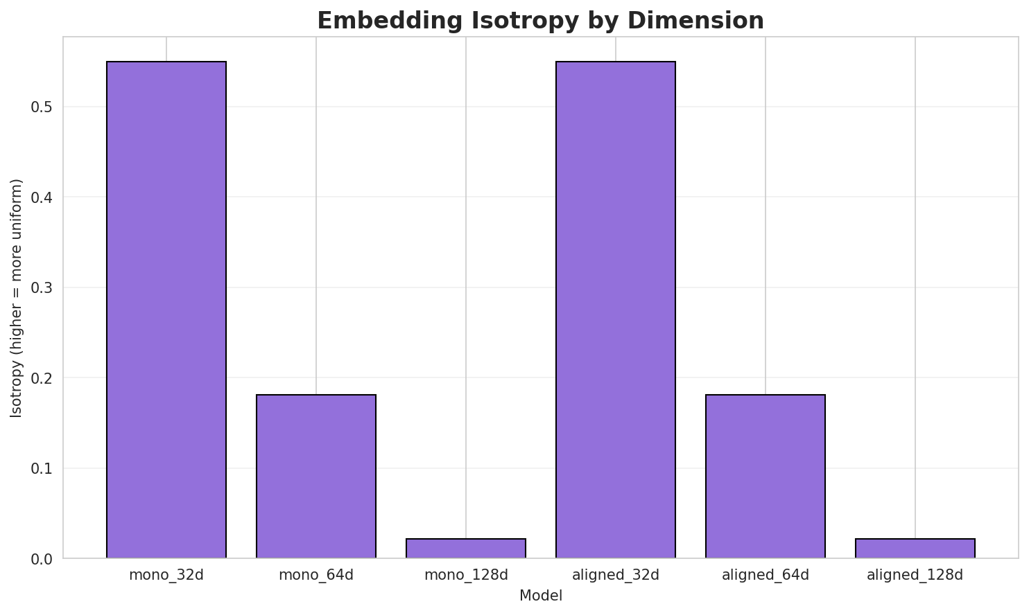
Model	Dimension	Isotropy	Semantic Density	Alignment R@1	Alignment R@10
mono_32d	32	0.5498 🏆	0.3626	N/A	N/A
mono_64d	64	0.1805	0.3661	N/A	N/A
mono_128d	128	0.0211	0.3761	N/A	N/A
aligned_32d	32	0.5498	0.3657	0.0260	0.1840
aligned_64d	64	0.1805	0.3550	0.0380	0.2240
aligned_128d	128	0.0211	0.3770	0.0480	0.2580

Key Findings

• Best Isotropy: mono_32d with 0.5498 (more uniform distribution)
• Semantic Density: Average pairwise similarity of 0.3671. Lower values indicate better semantic separation.
• Alignment Quality: Aligned models achieve up to 4.8% R@1 in cross-lingual retrieval.
• Recommendation: 128d aligned for best cross-lingual performance

---

6. Morphological Analysis (Experimental)

This section presents an automated morphological analysis derived from the statistical divergence between word-level and subword-level models. By analyzing where subword predictability spikes and where word-level coverage fails, we can infer linguistic structures without supervised data.

6.1 Productivity & Complexity

Metric	Value	Interpretation	Recommendation
Productivity Index	5.000	High morphological productivity	Reliable analysis
Idiomaticity Gap	0.386	High formulaic/idiomatic content	-

6.2 Affix Inventory (Productive Units)

These are the most productive prefixes and suffixes identified by sampling the vocabulary for global substitutability patterns. A unit is considered an affix if stripping it leaves a valid stem that appears in other contexts.

Productive Prefixes

Prefix	Examples
-t	tupono, taputapuatea, taraire
-p	pupuhi, pekanga, patukirikiri
-m	microsoft, momona, metcalf
-k	kāreti, kairangahau, kakabai
-ma	mashhad, marge, manukorihi
-h	honiara, homai, hūtāne
-a	arapohue, ano, ahiahi
-ta	taputapuatea, taraire, taradale

Productive Suffixes

Suffix	Examples
-a	honiara, pekanga, complexa
-i	homai, pupuhi, kāreti
-e	shore, hūtāne, arapohue
-ia	whakatakotohia, whakatuwheratia, incisapaesia
-s	reunionnais, carpodetus, press
-ga	pekanga, pānuitanga, patunga
-n	levin, susan, princeton
-o	werokoko, ano, tupono

6.3 Bound Stems (Lexical Roots)

Bound stems are high-frequency subword units that are semantically cohesive but rarely appear as standalone words. These often correspond to the 'core' of a word that requires inflection or derivation to be valid.

Stem	Cohesion	Substitutability	Examples
inga	1.83x	42 contexts	hinga, ringa, huinga
angi	1.91x	28 contexts	rangi, tangi, angitū
whak	1.96x	25 contexts	whaka, whakia, whakaū
rang	1.56x	58 contexts	range, rangi, ranga
hang	1.83x	28 contexts	hangā, hanga, hangai
akat	2.00x	20 contexts	akatea, whakatō, whakatū
enga	1.71x	34 contexts	henga, renga, awenga
onga	1.84x	24 contexts	longa, ponga, tonga
aita	1.70x	19 contexts	taita, vaita, whaita
taut	1.78x	14 contexts	tautau, tautoro, tautuhi
ngat	1.50x	19 contexts	ngati, ngata, ngatea
whan	1.81x	9 contexts	whano, whanga, whanau

6.4 Affix Compatibility (Co-occurrence)

This table shows which prefixes and suffixes most frequently co-occur on the same stems, revealing the 'stacking' rules of the language's morphology.

Prefix	Suffix	Frequency	Examples
-t	-a	203 words	temuka, tākaka
-p	-a	187 words	pūhonoiika, parawhenua
-k	-a	158 words	kopinga, kētia
-m	-a	123 words	maramara, mandiraja
-h	-a	122 words	hōhipera, henga
-t	-i	117 words	tāpoi, tuatini
-r	-a	109 words	rubra, robusta
-a	-a	93 words	ahumoana, akarana
-k	-i	89 words	kuki, koheriki
-m	-i	83 words	moanaui, mangaiti

6.5 Recursive Morpheme Segmentation

Using Recursive Hierarchical Substitutability, we decompose complex words into their constituent morphemes. This approach handles nested affixes (e.g., prefix-prefix-root-suffix).

Word	Suggested Split	Confidence	Stem
waikāretu	wa-i-kāretu	7.5	kāretu
matapouri	ma-ta-pouri	7.5	pouri
whakaratohia	whakarato-hi-a	7.5	hi
tamarangi	ta-ma-rangi	7.5	rangi
ngātokowaru	ngātokow-a-ru	7.5	a
whakatūnga	whakatū-ng-a	7.5	ng
huasolanum	hu-a-solanum	7.5	solanum
ulaanbaatar	ulaanbaat-a-r	7.5	a
joāeyeshvad	joāeyeshv-a-d	7.5	a
kaipūtaiao	ka-i-pūtaiao	7.5	pūtaiao
korerotia	korero-ti-a	7.5	ti
azərbaycan	azərbayc-a-n	7.5	a
tohatohahia	tohatoha-hi-a	7.5	hi
rokohanga	ro-ko-hanga	7.5	hanga
taharangi	ta-ha-rangi	7.5	rangi

6.6 Linguistic Interpretation

Automated Insight: The language Māori shows high morphological productivity. The subword models are significantly more efficient than word models, suggesting a rich system of affixation or compounding.

Note on Idiomaticity: The high Idiomaticity Gap suggests a large number of frequent multi-word expressions or formulaic sequences that are statistically distinct from their component parts.

---

7. Summary & Recommendations

Production Recommendations

Component	Recommended	Rationale
Tokenizer	64k BPE	Best compression (3.99x)
N-gram	2-gram	Lowest perplexity (171)
Markov	Context-4	Highest predictability (95.6%)
Embeddings	100d	Balanced semantic capture and isotropy

---

Appendix: Metrics Glossary & Interpretation Guide

This section provides definitions, intuitions, and guidance for interpreting the metrics used throughout this report.

Tokenizer Metrics

Compression Ratio

Definition: The ratio of characters to tokens (chars/token). Measures how efficiently the tokenizer represents text.

Intuition: Higher compression means fewer tokens needed to represent the same text, reducing sequence lengths for downstream models. A 3x compression means ~3 characters per token on average.

What to seek: Higher is generally better for efficiency, but extremely high compression may indicate overly aggressive merging that loses morphological information.

Average Token Length (Fertility)

Definition: Mean number of characters per token produced by the tokenizer.

Intuition: Reflects the granularity of tokenization. Longer tokens capture more context but may struggle with rare words; shorter tokens are more flexible but increase sequence length.

What to seek: Balance between 2-5 characters for most languages. Arabic/morphologically-rich languages may benefit from slightly longer tokens.

Unknown Token Rate (OOV Rate)

Definition: Percentage of tokens that map to the unknown/UNK token, indicating words the tokenizer cannot represent.

Intuition: Lower OOV means better vocabulary coverage. High OOV indicates the tokenizer encounters many unseen character sequences.

What to seek: Below 1% is excellent; below 5% is acceptable. BPE tokenizers typically achieve very low OOV due to subword fallback.

N-gram Model Metrics

Perplexity

Definition: Measures how "surprised" the model is by test data. Mathematically: 2^(cross-entropy). Lower values indicate better prediction.

Intuition: If perplexity is 100, the model is as uncertain as if choosing uniformly among 100 options at each step. A perplexity of 10 means effectively choosing among 10 equally likely options.

What to seek: Lower is better. Perplexity decreases with larger n-grams (more context). Values vary widely by language and corpus size.

Entropy

Definition: Average information content (in bits) needed to encode the next token given the context. Related to perplexity: perplexity = 2^entropy.

Intuition: High entropy means high uncertainty/randomness; low entropy means predictable patterns. Natural language typically has entropy between 1-4 bits per character.

What to seek: Lower entropy indicates more predictable text patterns. Entropy should decrease as n-gram size increases.

Coverage (Top-K)

Definition: Percentage of corpus occurrences explained by the top K most frequent n-grams.

Intuition: High coverage with few patterns indicates repetitive/formulaic text; low coverage suggests diverse vocabulary usage.

What to seek: Depends on use case. For language modeling, moderate coverage (40-60% with top-1000) is typical for natural text.

Markov Chain Metrics

Average Entropy

Definition: Mean entropy across all contexts, measuring average uncertainty in next-word prediction.

Intuition: Lower entropy means the model is more confident about what comes next. Context-1 has high entropy (many possible next words); Context-4 has low entropy (few likely continuations).

What to seek: Decreasing entropy with larger context sizes. Very low entropy (<0.1) indicates highly deterministic transitions.

Branching Factor

Definition: Average number of unique next tokens observed for each context.

Intuition: High branching = many possible continuations (flexible but uncertain); low branching = few options (predictable but potentially repetitive).

What to seek: Branching factor should decrease with context size. Values near 1.0 indicate nearly deterministic chains.

Predictability

Definition: Derived metric: (1 - normalized_entropy) × 100%. Indicates how deterministic the model's predictions are.

Intuition: 100% predictability means the next word is always certain; 0% means completely random. Real text falls between these extremes.

What to seek: Higher predictability for text generation quality, but too high (>98%) may produce repetitive output.

Vocabulary & Zipf's Law Metrics

Zipf's Coefficient

Definition: The slope of the log-log plot of word frequency vs. rank. Zipf's law predicts this should be approximately -1.

Intuition: A coefficient near -1 indicates the corpus follows natural language patterns where a few words are very common and most words are rare.

What to seek: Values between -0.8 and -1.2 indicate healthy natural language distribution. Deviations may suggest domain-specific or artificial text.

R² (Coefficient of Determination)

Definition: Measures how well the linear fit explains the frequency-rank relationship. Ranges from 0 to 1.

Intuition: R² near 1.0 means the data closely follows Zipf's law; lower values indicate deviation from expected word frequency patterns.

What to seek: R² > 0.95 is excellent; > 0.99 indicates near-perfect Zipf adherence typical of large natural corpora.

Vocabulary Coverage

Definition: Cumulative percentage of corpus tokens accounted for by the top N words.

Intuition: Shows how concentrated word usage is. If top-100 words cover 50% of text, the corpus relies heavily on common words.

What to seek: Top-100 covering 30-50% is typical. Higher coverage indicates more repetitive text; lower suggests richer vocabulary.

Word Embedding Metrics

Isotropy

Definition: Measures how uniformly distributed vectors are in the embedding space. Computed as the ratio of minimum to maximum singular values.

Intuition: High isotropy (near 1.0) means vectors spread evenly in all directions; low isotropy means vectors cluster in certain directions, reducing expressiveness.

What to seek: Higher isotropy generally indicates better-quality embeddings. Values > 0.1 are reasonable; > 0.3 is good. Lower-dimensional embeddings tend to have higher isotropy.

Average Norm

Definition: Mean magnitude (L2 norm) of word vectors in the embedding space.

Intuition: Indicates the typical "length" of vectors. Consistent norms suggest stable training; high variance may indicate some words are undertrained.

What to seek: Relatively consistent norms across models. The absolute value matters less than consistency (low std deviation).

Cosine Similarity

Definition: Measures angular similarity between vectors, ranging from -1 (opposite) to 1 (identical direction).

Intuition: Words with similar meanings should have high cosine similarity. This is the standard metric for semantic relatedness in embeddings.

What to seek: Semantically related words should score > 0.5; unrelated words should be near 0. Synonyms often score > 0.7.

t-SNE Visualization

Definition: t-Distributed Stochastic Neighbor Embedding - a dimensionality reduction technique that preserves local structure for visualization.

Intuition: Clusters in t-SNE plots indicate groups of semantically related words. Spread indicates vocabulary diversity; tight clusters suggest semantic coherence.

What to seek: Meaningful clusters (e.g., numbers together, verbs together). Avoid over-interpreting distances - t-SNE preserves local, not global, structure.

General Interpretation Guidelines

1. Compare within model families: Metrics are most meaningful when comparing models of the same type (e.g., 8k vs 64k tokenizer).
2. Consider trade-offs: Better performance on one metric often comes at the cost of another (e.g., compression vs. OOV rate).
3. Context matters: Optimal values depend on downstream tasks. Text generation may prioritize different metrics than classification.
4. Corpus influence: All metrics are influenced by corpus characteristics. Wikipedia text differs from social media or literature.
5. Language-specific patterns: Morphologically rich languages (like Arabic) may show different optimal ranges than analytic languages.

Visualizations Index

Visualization	Description
Tokenizer Compression	Compression ratios by vocabulary size
Tokenizer Fertility	Average token length by vocabulary
Tokenizer OOV	Unknown token rates
Tokenizer Total Tokens	Total tokens by vocabulary
N-gram Perplexity	Perplexity by n-gram size
N-gram Entropy	Entropy by n-gram size
N-gram Coverage	Top pattern coverage
N-gram Unique	Unique n-gram counts
Markov Entropy	Entropy by context size
Markov Branching	Branching factor by context
Markov Contexts	Unique context counts
Zipf's Law	Frequency-rank distribution with fit
Vocab Frequency	Word frequency distribution
Top 20 Words	Most frequent words
Vocab Coverage	Cumulative coverage curve
Embedding Isotropy	Vector space uniformity
Embedding Norms	Vector magnitude distribution
Embedding Similarity	Word similarity heatmap
Nearest Neighbors	Similar words for key terms
t-SNE Words	2D word embedding visualization
t-SNE Sentences	2D sentence embedding visualization
Position Encoding	Encoding method comparison
Model Sizes	Storage requirements
Performance Dashboard	Comprehensive performance overview

---

About This Project

Data Source

Models trained on wikipedia-monthly - a monthly snapshot of Wikipedia articles across 300+ languages.

Project

A project by Wikilangs - Open-source NLP models for every Wikipedia language.

Maintainer

Omar Kamali - Omneity Labs

Citation

If you use these models in your research, please cite:

@misc{wikilangs2025,
  author = {Kamali, Omar},
  title = {Wikilangs: Open NLP Models for Wikipedia Languages},
  year = {2025},
  doi = {10.5281/zenodo.18073153},
  publisher = {Zenodo},
  url = {https://huggingface.co/wikilangs}
  institution = {Omneity Labs}
}

License

MIT License - Free for academic and commercial use.

Links

• 🌐 Website: wikilangs.org
• 🤗 Models: huggingface.co/wikilangs
• 📊 Data: wikipedia-monthly
• 👤 Author: Omar Kamali
• 🤝 Sponsor: Featherless AI

---

Generated by Wikilangs Models Pipeline

Report Date: 2026-01-10 11:44:01