README.md

metadata

language: nqo
language_name: N’Ko
language_family: constructed_other
tags:
  - wikilangs
  - nlp
  - tokenizer
  - embeddings
  - n-gram
  - markov
  - wikipedia
  - feature-extraction
  - sentence-similarity
  - tokenization
  - n-grams
  - markov-chain
  - text-mining
  - fasttext
  - babelvec
  - vocabulous
  - vocabulary
  - monolingual
  - family-constructed_other
license: mit
library_name: wikilangs
pipeline_tag: text-generation
datasets:
  - omarkamali/wikipedia-monthly
dataset_info:
  name: wikipedia-monthly
  description: Monthly snapshots of Wikipedia articles across 300+ languages
metrics:
  - name: best_compression_ratio
    type: compression
    value: 4.453
  - name: best_isotropy
    type: isotropy
    value: 0.8251
  - name: vocabulary_size
    type: vocab
    value: 0
generated: 2026-01-10T00:00:00.000Z

N’Ko - Wikilangs Models

Comprehensive Research Report & Full Ablation Study

This repository contains NLP models trained and evaluated by Wikilangs, specifically on N’Ko Wikipedia data. We analyze tokenizers, n-gram models, Markov chains, vocabulary statistics, and word embeddings.

📋 Repository Contents

Models & Assets

• Tokenizers (8k, 16k, 32k, 64k)
• N-gram models (2, 3, 4, 5-gram)
• Markov chains (context of 1, 2, 3, 4 and 5)
• Subword N-gram and Markov chains
• Embeddings in various sizes and dimensions (aligned and unaligned)
• Language Vocabulary
• Language Statistics

Analysis and Evaluation

• 1. Tokenizer Evaluation
• 2. N-gram Model Evaluation
• 3. Markov Chain Evaluation
• 4. Vocabulary Analysis
• 5. Word Embeddings Evaluation
• 6. Morphological Analysis (Experimental)
• 7. Summary & Recommendations
• Metrics Glossary
• Visualizations Index

---

1. Tokenizer Evaluation

Results

Vocab Size	Compression	Avg Token Len	UNK Rate	Total Tokens
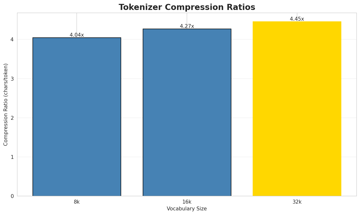
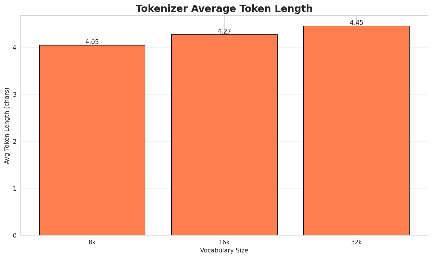
8k	4.044x	4.05	0.1822%	749,607
16k	4.267x	4.27	0.1923%	710,416
32k	4.453x 🏆	4.45	0.2007%	680,695

Tokenization Examples

Below are sample sentences tokenized with each vocabulary size:

Sample 1: ߘߊ߲ߘߊߟߌ ߓߏߟߏ߲ ߡߍ߲ ߣߊ߬ߕߊ ߦߋ߫ ߘߊ߲ߝߋ߲ ߞߍ߲ߘߍ ߥߟߴߊ߬ ߛߎ߭ ߟߎ߬ ߝߊ߬ߘߌ߬ ߛߓߏ ߓߣߊ߬ߦߊ߬ߣߍ߲ ߠߎ߬...

Vocab	Tokens	Count
8k	▁ߘߊ߲ߘߊߟߌ ▁ߓߏߟߏ߲ ▁ߡߍ߲ ▁ߣߊ߬ ߕߊ ▁ߦߋ߫ ▁ߘߊ߲ߝߋ߲ ▁ߞߍ߲ߘߍ ▁ߥߟߴߊ߬ ▁ߛߎ߭ ... (+10 more)	20
16k	▁ߘߊ߲ߘߊߟߌ ▁ߓߏߟߏ߲ ▁ߡߍ߲ ▁ߣߊ߬ߕߊ ▁ߦߋ߫ ▁ߘߊ߲ߝߋ߲ ▁ߞߍ߲ߘߍ ▁ߥߟߴߊ߬ ▁ߛߎ߭ ▁ߟߎ߬ ... (+9 more)	19
32k	▁ߘߊ߲ߘߊߟߌ ▁ߓߏߟߏ߲ ▁ߡߍ߲ ▁ߣߊ߬ߕߊ ▁ߦߋ߫ ▁ߘߊ߲ߝߋ߲ ▁ߞߍ߲ߘߍ ▁ߥߟߴߊ߬ ▁ߛߎ߭ ▁ߟߎ߬ ... (+7 more)	17

Sample 2: ߞߍ߲ߘߍߘߐߦߊ ߓߏߟߏ߲ ߡߍ߲ ߦߋ߫ ߞߏ߫ ߟߎ߫ ߞߊ߬ߙߊ߲߬ ߠߊ߫ ߸ ߡߍ߲ ߠߎ߬ ߦߋ߫ ߕߊ߬ ߟߊ߫ ߗߍ ߘߐ߫ ߓߐ߲ߛߐ߲ߢ...

Vocab	Tokens	Count
8k	▁ߞߍ߲ߘߍߘߐߦߊ ▁ߓߏߟߏ߲ ▁ߡߍ߲ ▁ߦߋ߫ ▁ߞߏ߫ ▁ߟߎ߫ ▁ߞߊ߬ߙߊ߲߬ ▁ߠߊ߫ ▁߸ ▁ߡߍ߲ ... (+11 more)	21
16k	▁ߞߍ߲ߘߍߘߐߦߊ ▁ߓߏߟߏ߲ ▁ߡߍ߲ ▁ߦߋ߫ ▁ߞߏ߫ ▁ߟߎ߫ ▁ߞߊ߬ߙߊ߲߬ ▁ߠߊ߫ ▁߸ ▁ߡߍ߲ ... (+11 more)	21
32k	▁ߞߍ߲ߘߍߘߐߦߊ ▁ߓߏߟߏ߲ ▁ߡߍ߲ ▁ߦߋ߫ ▁ߞߏ߫ ▁ߟߎ߫ ▁ߞߊ߬ߙߊ߲߬ ▁ߠߊ߫ ▁߸ ▁ߡߍ߲ ... (+10 more)	20

Sample 3: ߘߊ߲ߘߊߟߌ ߓߏߟߏ߲ ߡߍ߲ ߦߋ߫ ߝߘߏ߬ߓߊ߬ ߓߣߊ߬ ߞߟߊߞߟߊߕߊ ߟߎ߬ ߕߌߙߌ߲߫ ߠߊ߫.

Vocab	Tokens	Count
8k	▁ߘߊ߲ߘߊߟߌ ▁ߓߏߟߏ߲ ▁ߡߍ߲ ▁ߦߋ߫ ▁ߝߘߏ߬ߓߊ߬ ▁ߓߣߊ߬ ▁ߞߟߊߞߟߊ ߕߊ ▁ߟߎ߬ ▁ߕߌߙߌ߲߫ ... (+2 more)	12
16k	▁ߘߊ߲ߘߊߟߌ ▁ߓߏߟߏ߲ ▁ߡߍ߲ ▁ߦߋ߫ ▁ߝߘߏ߬ߓߊ߬ ▁ߓߣߊ߬ ▁ߞߟߊߞߟߊ ߕߊ ▁ߟߎ߬ ▁ߕߌߙߌ߲߫ ... (+2 more)	12
32k	▁ߘߊ߲ߘߊߟߌ ▁ߓߏߟߏ߲ ▁ߡߍ߲ ▁ߦߋ߫ ▁ߝߘߏ߬ߓߊ߬ ▁ߓߣߊ߬ ▁ߞߟߊߞߟߊߕߊ ▁ߟߎ߬ ▁ߕߌߙߌ߲߫ ▁ߠߊ߫ ... (+1 more)	11

Key Findings

• Best Compression: 32k achieves 4.453x compression
• Lowest UNK Rate: 8k with 0.1822% unknown tokens
• Trade-off: Larger vocabularies improve compression but increase model size
• Recommendation: 32k vocabulary provides optimal balance for production use

---

2. N-gram Model Evaluation

Results

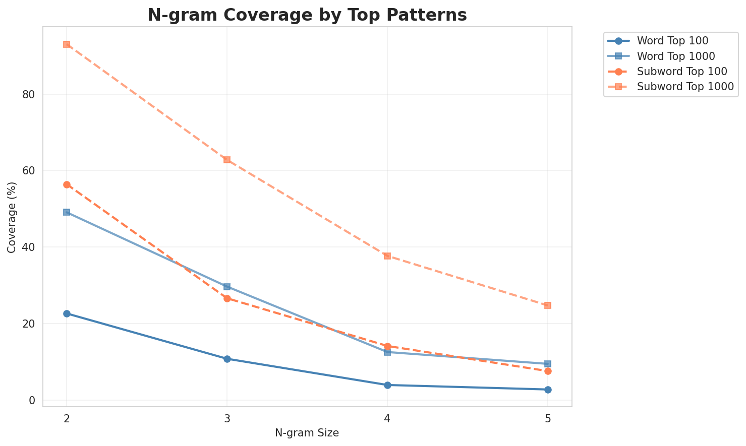
N-gram	Variant	Perplexity	Entropy	Unique N-grams	Top-100 Coverage	Top-1000 Coverage
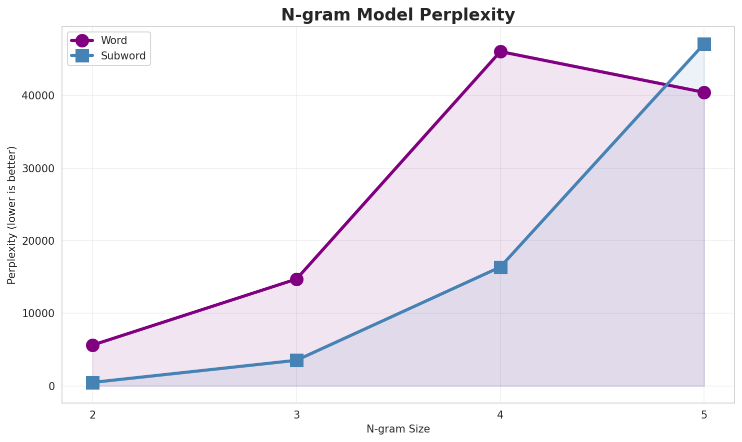
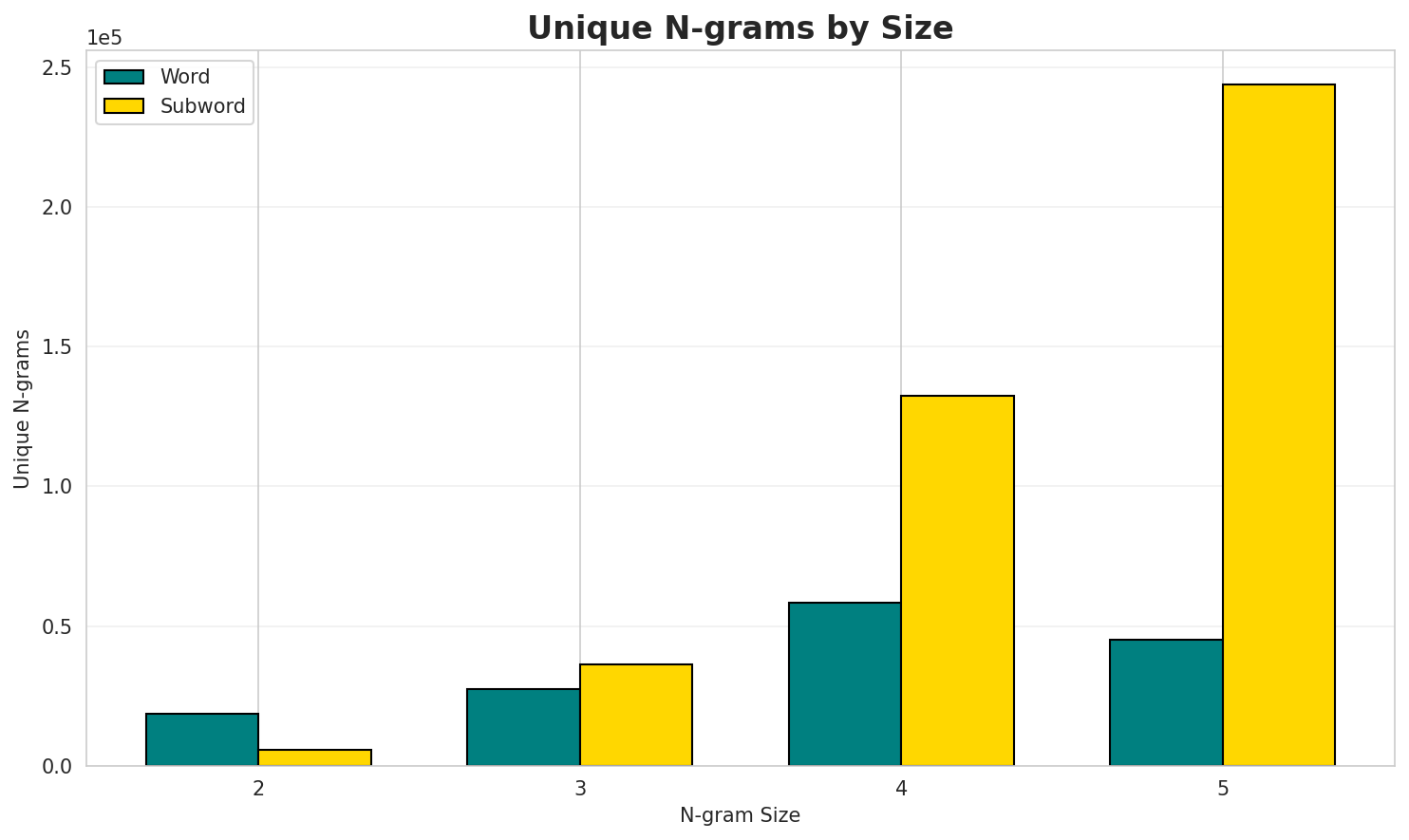
2-gram	Word	5,637	12.46	18,788	22.7%	49.1%
2-gram	Subword	492 🏆	8.94	5,832	56.4%	93.0%
3-gram	Word	14,726	13.85	27,596	10.9%	29.7%
3-gram	Subword	3,539	11.79	36,188	26.7%	62.8%
4-gram	Word	46,049	15.49	58,306	4.0%	12.6%
4-gram	Subword	16,382	14.00	132,351	14.2%	37.7%
5-gram	Word	40,435	15.30	45,104	2.8%	9.5%
5-gram	Subword	47,115	15.52	243,605	7.6%	24.8%

Top 5 N-grams by Size

2-grams (Word):

Rank	N-gram	Count
1	ߊ߬ ߣߌ߫	4,822
2	ߟߋ߬ ߘߌ߫	4,660
3	ߕߘߍ߬ ߦߋ߫	3,060
4	ߏ߬ ߟߋ	2,522
5	ߟߎ߬ ߟߊ߫	2,496

3-grams (Word):

Rank	N-gram	Count
1	ߘߏ߫ ߟߋ߬ ߘߌ߫	1,073
2	ߟߋ߬ ߘߌ߫ ߡߍ߲	752
3	ߟߋ߬ ߘߌ߫ ߊ߬	656
4	ߊ߬ ߣߌ߫ ߞߊ߬	633
5	ߘߐ߫ ߊ߬ ߣߌ߫	615

4-grams (Word):

Rank	N-gram	Count
1	ߘߏ߫ ߟߋ߬ ߘߌ߫ ߡߍ߲	257
2	ߟߋ߬ ߘߌ߫ ߊ߬ ߣߌ߫	165
3	ߏ߬ ߟߋ ߞߍ߫ ߘߊ߫	160
4	ߘߏ߫ ߟߋ߬ ߘߌ߫ ߊ߬	159
5	ߏ߬ ߡߍ߲ ߕߘߍ߬ ߦߋ߫	145

5-grams (Word):

Rank	N-gram	Count
1	ߦߋ߫ ߝߊ߬ߙߊ߲߬ߛߌ ߥߞߌߔߋߘߌߦߊ ߟߋ߬ ߡߊ߬	123
2	ߘߟߊߡߌ߬ߘߊ߬ߣߍ߲߫ ߦߋ߫ ߝߊ߬ߙߊ߲߬ߛߌ ߥߞߌߔߋߘߌߦߊ ߟߋ߬	118
3	ߣߌ߲߬ ߘߟߊߡߌ߬ߘߊ߬ߣߍ߲߫ ߦߋ߫ ߝߊ߬ߙߊ߲߬ߛߌ ߥߞߌߔߋߘߌߦߊ	111
4	ߘߏ߫ ߟߋ߬ ߘߌ߫ ߡߍ߲ ߦߋ߫	67
5	ߛߏ ߣߴߊ߬ ߡߙߊ߬ߘߊ߬ߘߎ߯ߟߊ ߘߏ߫ ߟߋ߬	65

2-grams (Subword):

Rank	N-gram	Count
1	_ ߞ	120,074
2	_ ߟ	100,993
3	_ ߘ	87,888
4	ߊ߬ _	83,535
5	ߊ߫ _	73,226

3-grams (Subword):

Rank	N-gram	Count
1	_ ߟ ߊ߫	32,190
2	ߟ ߊ߫ _	29,535
3	ߟ ߎ߬ _	23,162
4	_ ߞ ߊ߬	22,371
5	_ ߊ߬ _	21,289

4-grams (Subword):

Rank	N-gram	Count
1	_ ߟ ߊ߫ _	24,007
2	_ ߦ ߋ߫ _	19,822
3	_ ߟ ߎ߬ _	18,435
4	_ ߣ ߌ߫ _	17,034
5	_ ߟ ߋ߬ _	15,241

5-grams (Subword):

Rank	N-gram	Count
1	ߊ _ ߟ ߎ߬ _	6,974
2	_ ߞ ߵ ߊ߬ _	6,885
3	_ ߕ ߘ ߍ߬ _	6,060
4	_ ߟ ߋ߬ _ ߘ	5,988
5	_ ߟ ߊ߫ _ ߞ	5,476

Key Findings

• Best Perplexity: 2-gram (subword) with 492
• Entropy Trend: Decreases with larger n-grams (more predictable)
• Coverage: Top-1000 patterns cover ~25% of corpus
• Recommendation: 4-gram or 5-gram for best predictive performance

---

3. Markov Chain Evaluation

Results

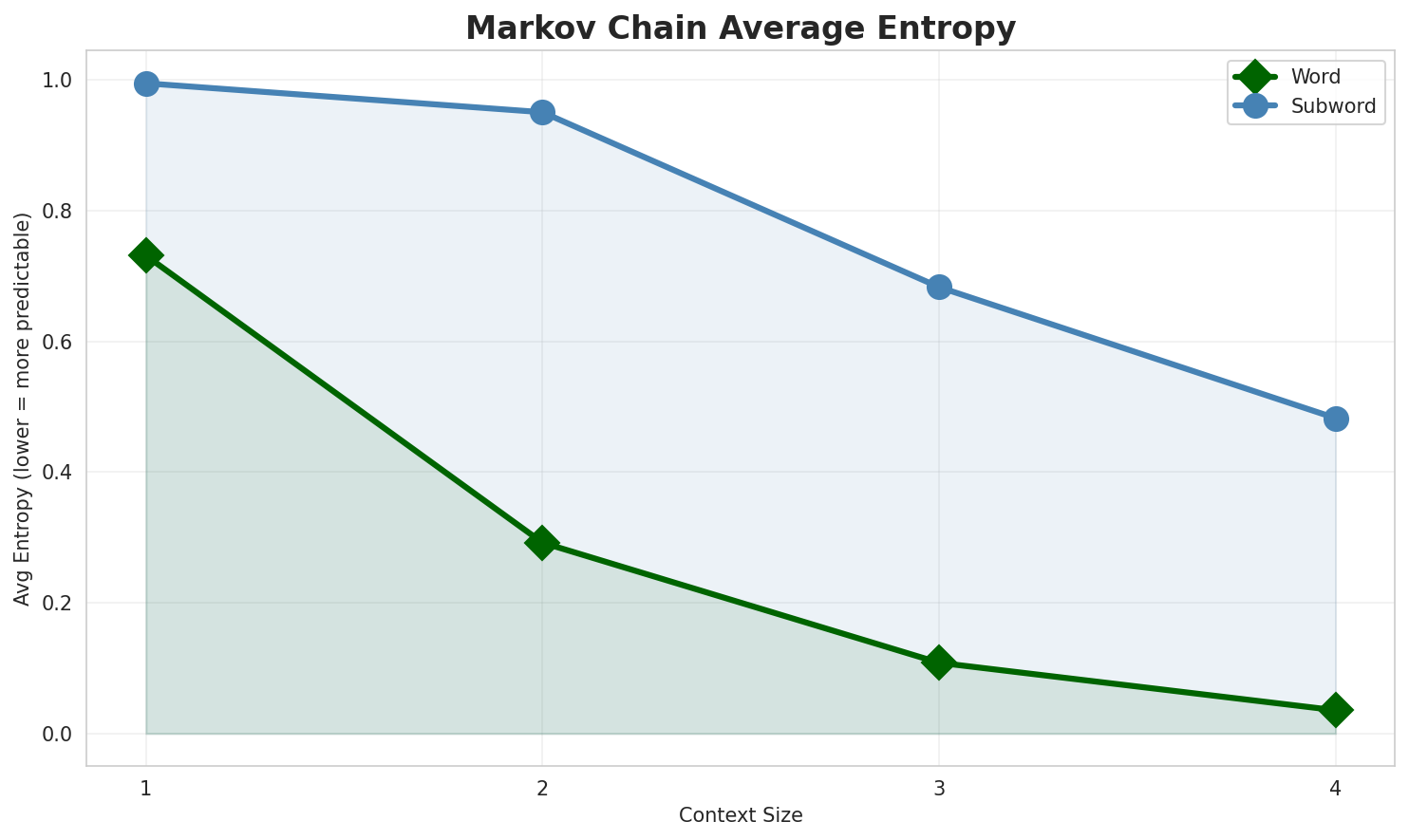
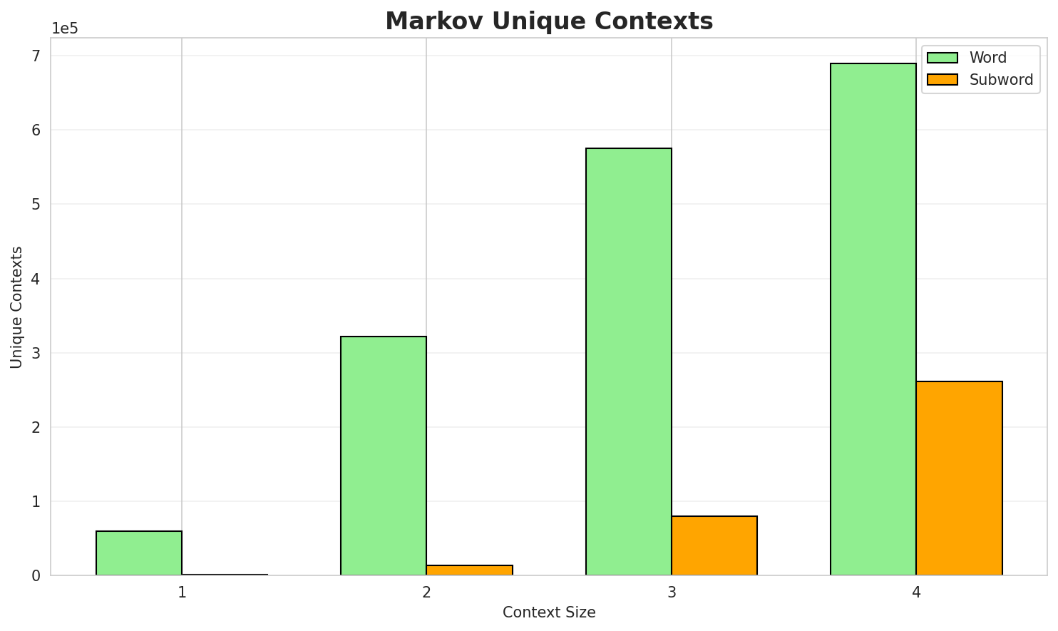
Context	Variant	Avg Entropy	Perplexity	Branching Factor	Unique Contexts	Predictability
1	Word	0.7313	1.660	5.40	59,713	26.9%
1	Subword	0.9951	1.993	10.03	1,379	0.5%
2	Word	0.2921	1.224	1.79	321,747	70.8%
2	Subword	0.9509	1.933	5.76	13,830	4.9%
3	Word	0.1083	1.078	1.20	575,482	89.2%
3	Subword	0.6832	1.606	3.28	79,681	31.7%
4	Word	0.0356 🏆	1.025	1.05	689,204	96.4%
4	Subword	0.4827	1.397	2.20	261,417	51.7%

Generated Text Samples (Word-based)

Below are text samples generated from each word-based Markov chain model:

Context Size 1:

1. ߟߊ߫ ߓߌ߬ߟߊ߬ߢߐ߲߰ߠߊ ߃ߟߋ߬ ߘߐ߫ ߊ߬ ߕߌ߲߬ߞߎߘߎ߲ ߘߐ߫ ߣߴߊ߬ߟߎ߫ ߕߘߍ߬ ߘߊ߫ ߓߏ߲ ߠߊ߫ ߝߊ߬ߙߊ߲߬ߛߌ߫ ߟߊ߫ ߞߎߡߊߘߋ߲ ߘߏ߫
2. ߊ߬ ߖߘߍ߬ ߟߊ߫ ߊ߬ ߣߴߊ߬ ߥߟߎ߬ߥߟߎ ߟߎ߬ ߡߊ߫ ߡߊ߰ ߘߴߊ߬ߟߎ߫ ߡߊ߬ ߞߵߊ߬ ߘߊߡߌ߬ߣߊ߬ ߞߏ߫ ߌ ߝߣߊ߫
3. ߦߋ߫ ߜߟߊ߬ߜߟߊ߫ ߘߌ߫ ߟߊ߫ ߕߓߌߟߌ߫ ߕߙߏߞߏ ߟߎ߬ ߣߴߊ߬ ߘߟߊߡߌ߬ߘߊ߬ߣߍ߲ ߘߴߊ߬ ߦߋ߫ ߕߌ߲߬ߞߎ߬ߘߎ߲߬ ߇߲ ߞߊ߬ ߛߎ߲ߞߊߙߏ ߓߊ߲

Context Size 2:

1. ߊ߬ ߣߌ߫ ߞߐ ߟߊ߫ ߏ߬ ߞߵߊ߬ ߛߐ߫ ߟߌ߲߬ߖߌ߯ߟߌ ߟߊ߫ ߞߊ߲ߘߦߊ ߣߌ߫ ߟߊ߬ߟߌ߬ߟߌ ߟߋ߬ ߓߟߏ߫ ߓߊ ߏ߬ ߟߋ
2. ߟߋ߬ ߘߌ߫ ߟߊߓߋ߫ ߕߌ߲߬ߞߎߘߎ߲ ߘߐ߫ ߊ߬ ߟߊ߫ ߢߣߊߡߦߊ ߘߐ߫ ߛߔߑߙߌ߲ߜ߭ߛ ߔߊߦߑߣߌ߫ ߞߊ߲ߕߌ߮ ߟߌߓߋߙߌߦߞߊ
3. ߕߘߍ߬ ߦߋ߫ ߡߐ߰ ߟߎ߫ ߟߋ߬ ߞߘߊߡߊ߫ ߞߊ߬ ߝߊ߬ߛߏ߬ߟߊ߬ߞߊ ߘߐ߬ߕߊߡߌ߲ ߟߊ߬ߟߌ߰ߟߌ ߓߌ߬ߟߊ߬ ߘߊ߫ ߛߋ߲߬ߠߊ߫ ߕߎߟߊߝߌ߲ ߂߈ ߡߊ߬ ߕߙߍߛ...

Context Size 3:

1. ߘߏ߫ ߟߋ߬ ߘߌ߫ ߞߊ߬ ߝߘߊ߫ ߊߘߐߟߝ ߤߌߕߑߟߍߙ ߟߊ߫ ߘߊߘߐߥߛߊ ߞߛߊ߬ߓߌ ߡߊ߬ ߊ߬ ߞߵߊ߬ ߟߊ߫ ߞߟߏߞߕߏߦߊ ߏ߬ ߛߐ߬ߘߐ߲߬ ߋߙߐߔߎߞߊ
2. ߟߋ߬ ߘߌ߫ ߡߍ߲ ߣߌ߫ ߥߙߐ߬ߞߘߐ߫ ߝߊ߭ߡߘߎ߬ ߟߎ߫ ߘߍ߬ ߘߊ߫ ߞߊ߬ ߣߏߙߊߛߏߓߊ߫ ߘߟߊߛߌ߰ ߞߊ߬ ߟߊ߬ߥߛߊ߫ ߛߐ߬ߘߐ߲߫ ߞߊ߬ߙߊ߲߬ߕߏ߲߫ ߞߎ...
3. ߟߋ߬ ߘߌ߫ ߊ߬ ߥߟߏߘߊ ߟߋ߬ ߟߊ߫ ߏ߬ ߞߍ ߊ߬ ߓߐ߫ ߘߴߊ߬ ߟߐ߬ߘߎ߮ ߘߐ߫ ߊ߬ ߓߊ߯ߙߘߊ߫ ߘߊߺߊ߳ߑߥߟߊ߫ ߌߡߊ߰ߡߎ߲߫ ߣߌ߫

Context Size 4:

1. ߘߏ߫ ߟߋ߬ ߘߌ߫ ߡߍ߲ ߕߘߍ߬ ߦߋ߫ ߞߘߏߥߊߙߌ߫ ߕߟߋ߬ߓߋ ߥߙߏ߬ߘߎ߮ ߣߌ߫ ߕߐ߬ߙߐ߲߬ ߣߌ߫ ߝߏߟߏ߲ߣߍ߲߬ߜߍ߫ ߟߎ߫ ߣߴߊ߬ߟߎ߬ ߟߊߡߌߣߌ߲ ߞߊ...
2. ߟߋ߬ ߘߌ߫ ߊ߬ ߣߌ߫ ߞߴߏ߬ ߥߊ߯ߕߌ߫ ߞߋߟߋ߲ ߠߊ߫ ߞߏ߫ ߞߍߒߞߊ߲ߠߌ߲߫ ߘߍ߰ߜߍ ߘߏ߫ ߘߌ߫ ߓߌ߬ߟߊ߫ ߛߋ߲߬ߠߊ߫ ߥߙߏ߬ߘߎ߮ ߘߐ߫ ߏߔߋߙߊߛ߭...
3. ߏ߬ ߟߋ ߞߍ߫ ߘߊ߫ ߖߋ߬ߟߌ ߛߎ߯ߦߊ߫ ߞߎߘߊ߫ ߟߊߘߊ߲ߣߍ߲ ߘߌ߫ ߡߊ߲߬ߘߋ߲߫ ߛߊ߫ ߛߏ߲߬ߖߘߊ߫ ߛߌ߰ߣߍ߲ ߏ߬ ߞߍ߫ ߘߊ߫ ߡߊ߲߬ߘߋ߲߬ߞߊ ߟߎ߬...

Generated Text Samples (Subword-based)

Below are text samples generated from each subword-based Markov chain model:

Context Size 1:

1. _ߟߎ߬_ߖߙߊ߲߬ߕߎ߲߬_ߟߐ߬ߘߏ߬ߘߌ߫
2. ߟߋߘߺߋ߬ߓߍߘߌ߫_ߟߌ_ߓߍߟ
3. ߞߵߊ߬_ߞߏ߬_ߊ߬_ߘߎ߲ߣߴߊ߬_ߛ

Context Size 2:

1. _ߞߛߐߟߊ_ߓߟߏ߫_ߣߌ߫_ߊ߬ߟߌ
2. _ߟߊ߫_߸_ߤߙߊ_ߕߊ_ߓߘߍ߬ߣ
3. _ߘߐ߫_ߞߊ߬ߦߊ_ߟߌ߲ߓߊ߫_ߡߴߊ߬

Context Size 3:

1. _ߟߊ߫_ߝߍ߫_ߦߋ߲߬_ߠߋ߬_ߦߋ߫_ߓߊ߯
2. ߟߊ߫_ߞߏ߫_ߡߐ߱_ߟߎ߬_ߡߐ߰_ߡߴߊ߬
3. ߟߎ߬_ߖߍ߬ߘߍ_ߛߌ߰_ߗߋߘߊ_ߣߌ߲߬

Context Size 4:

1. _ߟߊ߫_ߕߟߋ߬ߓߋ_ߘߐ߫߸_ߗߍ߭_ߡߛ
2. _ߦߋ߫_ߡߊ߬ߟߌ_ߞߐߛߊߦߌߡߊ_ߏ߬
3. _ߟߎ߬_ߟߊ߫_ߝߛߊߦߌ߫߸_ߓߎߙߎ߲ߘ

Key Findings

• Best Predictability: Context-4 (word) with 96.4% predictability
• Branching Factor: Decreases with context size (more deterministic)
• Memory Trade-off: Larger contexts require more storage (261,417 contexts)
• Recommendation: Context-3 or Context-4 for text generation

---

4. Vocabulary Analysis

Statistics

Metric	Value
Vocabulary Size	24,726
Total Tokens	758,182
Mean Frequency	30.66
Median Frequency	3
Frequency Std Dev	453.65

Most Common Words

Rank	Word	Frequency
1	ߟߊ߫	32,133
2	ߊ߬	22,764
3	ߦߋ߫	20,445
4	ߘߌ߫	19,370
5	ߟߎ߬	19,254
6	ߘߐ߫	18,014
7	ߣߌ߫	17,228
8	ߏ߬	16,452
9	ߟߋ߬	15,933
10	ߞߊ߬	15,452

Least Common Words (from vocabulary)

Rank	Word	Frequency
1	ߛߌߦߋߙߊߟߋߦߐ߲߫	2
2	ߡߊ߲߬ߜ߭ߊ߫	2
3	ߛߏߟߌߡߊ߫	2
4	ߦߊ߬ߟߎ߲߬ߞߊ߫	2
5	ߞߏߦߌ߲ߘߎ߯	2
6	ߞߊߦߌߟߊ߯ߤߎ߲߫	2
7	ߥߙߏ߬ߘߜ߭ߎ	2
8	ߢߐ߲ߜ߭ߐ߲	2
9	ep	2
10	ߣߊߣߌ	2

Zipf's Law Analysis

Metric	Value
Zipf Coefficient	1.1458
R² (Goodness of Fit)	0.995876
Adherence Quality	excellent

Coverage Analysis

Top N Words	Coverage
Top 100	53.3%
Top 1,000	76.5%
Top 5,000	90.4%
Top 10,000	95.0%

Key Findings

• Zipf Compliance: R²=0.9959 indicates excellent adherence to Zipf's law
• High Frequency Dominance: Top 100 words cover 53.3% of corpus
• Long Tail: 14,726 words needed for remaining 5.0% coverage

---

5. Word Embeddings Evaluation

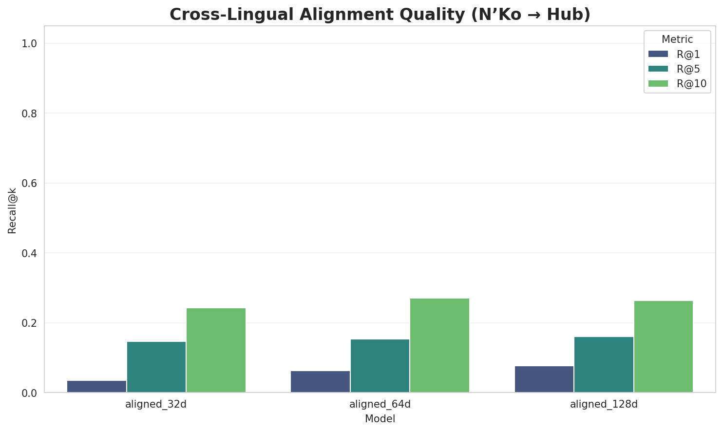
5.1 Cross-Lingual Alignment

5.2 Model Comparison

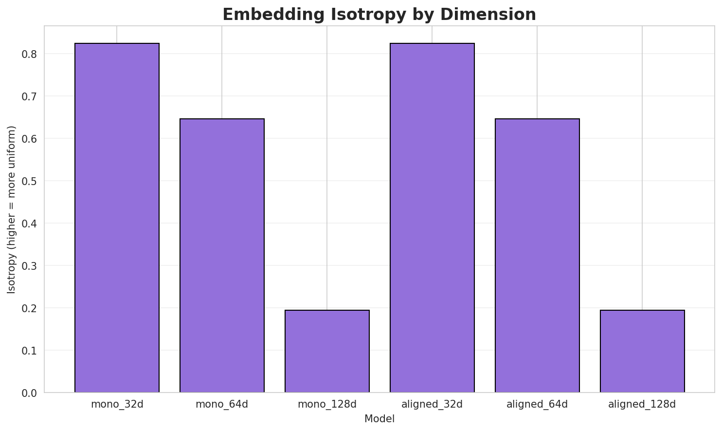
Model	Dimension	Isotropy	Semantic Density	Alignment R@1	Alignment R@10
mono_32d	32	0.8251 🏆	0.3375	N/A	N/A
mono_64d	64	0.6469	0.2857	N/A	N/A
mono_128d	128	0.1940	0.2840	N/A	N/A
aligned_32d	32	0.8251	0.3411	0.0347	0.2431
aligned_64d	64	0.6469	0.2880	0.0625	0.2708
aligned_128d	128	0.1940	0.2779	0.0764	0.2639

Key Findings

• Best Isotropy: mono_32d with 0.8251 (more uniform distribution)
• Semantic Density: Average pairwise similarity of 0.3024. Lower values indicate better semantic separation.
• Alignment Quality: Aligned models achieve up to 7.6% R@1 in cross-lingual retrieval.
• Recommendation: 128d aligned for best cross-lingual performance

---

6. Morphological Analysis (Experimental)

This section presents an automated morphological analysis derived from the statistical divergence between word-level and subword-level models. By analyzing where subword predictability spikes and where word-level coverage fails, we can infer linguistic structures without supervised data.

6.1 Productivity & Complexity

Metric	Value	Interpretation	Recommendation
Productivity Index	5.000	High morphological productivity	Reliable analysis
Idiomaticity Gap	-0.615	Low formulaic content	-

6.2 Affix Inventory (Productive Units)

These are the most productive prefixes and suffixes identified by sampling the vocabulary for global substitutability patterns. A unit is considered an affix if stripping it leaves a valid stem that appears in other contexts.

Productive Prefixes

Prefix	Examples
-ߞ	ߞߏߔߣߌ߲߬, ߞߴߊ߬ߟߌ߬ߞߊ߰ߓߊ߬, ߞߐ߰ߖߌ߬ߘߟߊ߬
-ߛ	ߛߍ߲ߕߊ߬, ߛߐ߲ߞߐ߫, ߛߊ߲ߡߊߝߋ߲
-ߟߊ	ߟߊߛߴߊ߬, ߟߊ߬ߡߙߊ߬ߟߌ, ߟߊߡߐ߰
-ߡߊ	ߡߊ߬ߣߌ߲߬ߝߐߛߐ߲, ߡߊ߬ߘߌ߬ߡߌ߲߬ߣߌ߲, ߡߊ߯
-ߓ	ߓߍ߲߬ߓߊ߬ߟߌ߬ߦߊ߬, ߓߊߓߋ߬, ߓߛߌ߬ߞߌ߬ߟߌ
-ߘ	ߘߎ߰ߓߊ߫, ߘߐߜߍߕߊ, ߘߐ߲߬ߓߏ߲
-ߡ	ߡߍ߲ߘߌߦߊ߫, ߡߊ߬ߣߌ߲߬ߝߐߛߐ߲, ߡߊ߬ߘߌ߬ߡߌ߲߬ߣߌ߲
-ߕ	ߕߙߐߝߍ߬, ߕߎ߲߯ߣߍ߲߫, ߕߍ߬ߘߵߊ߬ߟߎ߬

Productive Suffixes

Suffix	Examples
-ߊ	ߝߊ߬ߘߌ߬ߜߊ, ߞߊ߬ߙߊ߲߬ߡߐ߰ߓߊ, ߖߊ߯ߓߊߟߌߦߊ
-ߌ	ߓߛߌ߬ߞߌ߬ߟߌ, ߜߏ߬ߞߌ, ߣߌ߬ߣߌ߬ߟߌ
-ߦߊ	ߖߊ߯ߓߊߟߌߦߊ, ߗߍ߬ߣߌ߫ߡߛߏ߬ߦߊ, ߣߝߊ߬ߢߐ߰ߦߊ
-ߟߌ	ߓߛߌ߬ߞߌ߬ߟߌ, ߣߌ߬ߣߌ߬ߟߌ, ߟߊ߬ߡߙߊ߬ߟߌ
-ߟߊ	ߛߋߟߊ, ߟߊߓߌ߬ߟߊ, ߥߎߟߊ
-ߞߊ	ߞߊ߲ߞߊ, ߓߌߋߟߏߙߎߛߌߞߊ, ߊߡߋߙߞߌߟߞߊ
-ߏ	ߟߊ߬ߖߊ߲ߞߏ, ߡߊ߬ߞߊߝߏ, ߦߙߏ
-ߡߊ	ߡߐ߬ߟߐ߲߬ߡߊ, ߖߛߐߡߊ, ߝߊߕߎߡߊ

6.3 Bound Stems (Lexical Roots)

Bound stems are high-frequency subword units that are semantically cohesive but rarely appear as standalone words. These often correspond to the 'core' of a word that requires inflection or derivation to be valid.

Stem	Cohesion	Substitutability	Examples
ߝߙߌߞ	2.30x	19 contexts	ߊߝߙߌߞ, ߊߝߙߌߞߊ, ߊߝߙߌߞߊ߲
ߡߋߙߌ	2.17x	14 contexts	ߊߡߋߙߌߞ, ߋߡߋߙߌߞ, ߊߡߋߙߌߞߌ
ߞߎߡߘ	2.28x	12 contexts	ߞߎߡߘߊ, ߞߎߡߘߊ߫, ߘߐ߫ߞߎߡߘߊ
ߊߙߊߓ	2.14x	14 contexts	ߊߙߊߓߎ, ߊߙߊߓߍߟ, ߊߙߊߓߎ߫
ߟߌߦߊ	1.67x	30 contexts	ߦߟߌߦߊ, ߜߟߌߦߊ, ߞߊߟߌߦߊ
ߞߏߟߊ	1.88x	20 contexts	ߞߏߟߊ߫, ߞߏߟߊߕߍ, ߣߌߞߏߟߊ
ߊߟߌߦ	1.85x	14 contexts	ߞߊߟߌߦߊ, ߓߊߟߌߦߊ, ߥߊߟߌߦߊ
ߟߌߡߊ	1.48x	25 contexts	ߟߌߡߊ߫, ߦߟߌߡߊ, ߥߊߟߌߡߊ
ߦߊߟߌ	1.72x	15 contexts	ߖߏߦߊߟߌ, ߗߋߦߊߟߌ, ߗߋߦߊߟߌ߫
ߓߟߏߡ	1.64x	16 contexts	ߓߟߏߡߊ, ߓߟߏߡߐ, ߓߟߏߡߐ߮
ߊߟߏߡ	2.36x	6 contexts	ߊߟߏߡߊ߲, ߊߟߏߡߊ߲߫, ߊߟߏߡߊߦߌ߲
ߛߓߍߟ	1.65x	11 contexts	ߛߓߍߟߌ, ߛߓߍߟߊ, ߛߓߍߟߊ߲

6.4 Affix Compatibility (Co-occurrence)

This table shows which prefixes and suffixes most frequently co-occur on the same stems, revealing the 'stacking' rules of the language's morphology.

Prefix	Suffix	Frequency	Examples
-ߞ	-ߊ	158 words	ߞߊ߲߬ߖߊ, ߞߐ߯ߟߕߊ
-ߛ	-ߊ	102 words	ߛߦߊ, ߛߏ߯ߡߦߊ
-ߘ	-ߊ	85 words	ߘߐ߲߬ߖߊ߬ߓߊ, ߘߐߜߟߌߦߊ
-ߓ	-ߊ	73 words	ߓߏ߬ߢߊ, ߓߋߕߊ
-ߝ	-ߊ	63 words	ߝߎߥߟߊ, ߝߘߏ߬ߓߊ߬ߦߊ
-ߟߊ	-ߌ	53 words	ߟߊߕߊ߯ߟߌ, ߟߊ߬ߕߊ߲߬ߞߊ߬ߟߌ
-ߞ	-ߦߊ	48 words	ߞߏ߲߬ߓߏ߬ߦߊ, ߞߌ߬ߣߊ߬ߦߊ
-ߕ	-ߊ	43 words	ߕߊ߲ߓߊ߲ߞߕߐߦߊ, ߕߍߟߐߦߊ
-ߞ	-ߌ	41 words	ߞߎ߬ߙߊ߬ߦߌ߬ߛߌ, ߞߊ߲ߠߊߓߌߟߊߟߌ
-ߘ	-ߌ	40 words	ߘߝߐߟߌ, ߘߝߊߟߌ

6.5 Recursive Morpheme Segmentation

Using Recursive Hierarchical Substitutability, we decompose complex words into their constituent morphemes. This approach handles nested affixes (e.g., prefix-prefix-root-suffix).

Word	Suggested Split	Confidence	Stem
ߛߊߡߊߞߎߟߎ߲	ߛߊ-ߡߊ-ߞߎߟߎ߲	7.5	ߞߎߟߎ߲
ߖߙߊߘߛߌߕߙߊߦߊ	ߖߙߊߘߛߌߕߙ-ߊ-ߦߊ	7.5	ߊ
ߘߟߊߡߌ߬ߣߊ߬	ߘ-ߟߊ-ߡߌ߬ߣߊ߬	7.5	ߡߌ߬ߣߊ߬
ߊߙߑߛ߭ߌߣߊߙ	ߊߙߑߛ߭ߌߣ-ߊ-ߙ	7.5	ߊ
ߘߊߟߞߊߟߌߦߊ	ߘߊ-ߟ-ߞߊߟߌߦߊ	7.5	ߞߊߟߌߦߊ
ߓߟߏߟߊߓߊ߯ߙߊ߫	ߓߟߏ-ߟߊ-ߓߊ߯ߙߊ߫	7.5	ߓߊ߯ߙߊ߫
ߦߟߌߓߌߟߊߟߌ	ߦߟߌߓߌߟ-ߊ-ߟߌ	7.5	ߊ
ߓߟߏߡߊߕߌߢߍߣߍ߲	ߓߟߏ-ߡߊ-ߕߌߢߍߣߍ߲	7.5	ߕߌߢߍߣߍ߲
ߣߊߡߎ߲ߘߐߞߏ	ߣߊߡߎ߲-ߘߐ-ߞߏ	7.5	ߘߐ
ߝߘߊߢߐ߲߯ߦߊ	ߝ-ߘߊ-ߢߐ߲߯ߦߊ	7.5	ߢߐ߲߯ߦߊ
ߦߟߍ߬ߡߊ߲߬ߓߊߟߌ	ߦߟߍ߬ߡߊ߲߬ߓ-ߊ-ߟߌ	7.5	ߊ
ߦߌߟߡߊߦߊߟߌ	ߦߌߟߡߊ-ߦߊ-ߟߌ	6.0	ߦߌߟߡߊ
ߝߘߎߓߊߟߌߦߊ	ߝ-ߘߎ-ߓߊߟߌߦߊ	6.0	ߓߊߟߌߦߊ
ߞߐ߲ߛߐ߲ߦߊߟߌ	ߞߐ߲ߛߐ߲-ߦߊ-ߟߌ	6.0	ߞߐ߲ߛߐ߲
ߛߏ߯ߙߏߟߌߟߊ	ߛߏ߯ߙߏ-ߟߌ-ߟߊ	6.0	ߛߏ߯ߙߏ

6.6 Linguistic Interpretation

Automated Insight: The language N’Ko shows high morphological productivity. The subword models are significantly more efficient than word models, suggesting a rich system of affixation or compounding.

---

7. Summary & Recommendations

Production Recommendations

Component	Recommended	Rationale
Tokenizer	32k BPE	Best compression (4.45x)
N-gram	2-gram	Lowest perplexity (492)
Markov	Context-4	Highest predictability (96.4%)
Embeddings	100d	Balanced semantic capture and isotropy

---

Appendix: Metrics Glossary & Interpretation Guide

This section provides definitions, intuitions, and guidance for interpreting the metrics used throughout this report.

Tokenizer Metrics

Compression Ratio

Definition: The ratio of characters to tokens (chars/token). Measures how efficiently the tokenizer represents text.

Intuition: Higher compression means fewer tokens needed to represent the same text, reducing sequence lengths for downstream models. A 3x compression means ~3 characters per token on average.

What to seek: Higher is generally better for efficiency, but extremely high compression may indicate overly aggressive merging that loses morphological information.

Average Token Length (Fertility)

Definition: Mean number of characters per token produced by the tokenizer.

Intuition: Reflects the granularity of tokenization. Longer tokens capture more context but may struggle with rare words; shorter tokens are more flexible but increase sequence length.

What to seek: Balance between 2-5 characters for most languages. Arabic/morphologically-rich languages may benefit from slightly longer tokens.

Unknown Token Rate (OOV Rate)

Definition: Percentage of tokens that map to the unknown/UNK token, indicating words the tokenizer cannot represent.

Intuition: Lower OOV means better vocabulary coverage. High OOV indicates the tokenizer encounters many unseen character sequences.

What to seek: Below 1% is excellent; below 5% is acceptable. BPE tokenizers typically achieve very low OOV due to subword fallback.

N-gram Model Metrics

Perplexity

Definition: Measures how "surprised" the model is by test data. Mathematically: 2^(cross-entropy). Lower values indicate better prediction.

Intuition: If perplexity is 100, the model is as uncertain as if choosing uniformly among 100 options at each step. A perplexity of 10 means effectively choosing among 10 equally likely options.

What to seek: Lower is better. Perplexity decreases with larger n-grams (more context). Values vary widely by language and corpus size.

Entropy

Definition: Average information content (in bits) needed to encode the next token given the context. Related to perplexity: perplexity = 2^entropy.

Intuition: High entropy means high uncertainty/randomness; low entropy means predictable patterns. Natural language typically has entropy between 1-4 bits per character.

What to seek: Lower entropy indicates more predictable text patterns. Entropy should decrease as n-gram size increases.

Coverage (Top-K)

Definition: Percentage of corpus occurrences explained by the top K most frequent n-grams.

Intuition: High coverage with few patterns indicates repetitive/formulaic text; low coverage suggests diverse vocabulary usage.

What to seek: Depends on use case. For language modeling, moderate coverage (40-60% with top-1000) is typical for natural text.

Markov Chain Metrics

Average Entropy

Definition: Mean entropy across all contexts, measuring average uncertainty in next-word prediction.

Intuition: Lower entropy means the model is more confident about what comes next. Context-1 has high entropy (many possible next words); Context-4 has low entropy (few likely continuations).

What to seek: Decreasing entropy with larger context sizes. Very low entropy (<0.1) indicates highly deterministic transitions.

Branching Factor

Definition: Average number of unique next tokens observed for each context.

Intuition: High branching = many possible continuations (flexible but uncertain); low branching = few options (predictable but potentially repetitive).

What to seek: Branching factor should decrease with context size. Values near 1.0 indicate nearly deterministic chains.

Predictability

Definition: Derived metric: (1 - normalized_entropy) × 100%. Indicates how deterministic the model's predictions are.

Intuition: 100% predictability means the next word is always certain; 0% means completely random. Real text falls between these extremes.

What to seek: Higher predictability for text generation quality, but too high (>98%) may produce repetitive output.

Vocabulary & Zipf's Law Metrics

Zipf's Coefficient

Definition: The slope of the log-log plot of word frequency vs. rank. Zipf's law predicts this should be approximately -1.

Intuition: A coefficient near -1 indicates the corpus follows natural language patterns where a few words are very common and most words are rare.

What to seek: Values between -0.8 and -1.2 indicate healthy natural language distribution. Deviations may suggest domain-specific or artificial text.

R² (Coefficient of Determination)

Definition: Measures how well the linear fit explains the frequency-rank relationship. Ranges from 0 to 1.

Intuition: R² near 1.0 means the data closely follows Zipf's law; lower values indicate deviation from expected word frequency patterns.

What to seek: R² > 0.95 is excellent; > 0.99 indicates near-perfect Zipf adherence typical of large natural corpora.

Vocabulary Coverage

Definition: Cumulative percentage of corpus tokens accounted for by the top N words.

Intuition: Shows how concentrated word usage is. If top-100 words cover 50% of text, the corpus relies heavily on common words.

What to seek: Top-100 covering 30-50% is typical. Higher coverage indicates more repetitive text; lower suggests richer vocabulary.

Word Embedding Metrics

Isotropy

Definition: Measures how uniformly distributed vectors are in the embedding space. Computed as the ratio of minimum to maximum singular values.

Intuition: High isotropy (near 1.0) means vectors spread evenly in all directions; low isotropy means vectors cluster in certain directions, reducing expressiveness.

What to seek: Higher isotropy generally indicates better-quality embeddings. Values > 0.1 are reasonable; > 0.3 is good. Lower-dimensional embeddings tend to have higher isotropy.

Average Norm

Definition: Mean magnitude (L2 norm) of word vectors in the embedding space.

Intuition: Indicates the typical "length" of vectors. Consistent norms suggest stable training; high variance may indicate some words are undertrained.

What to seek: Relatively consistent norms across models. The absolute value matters less than consistency (low std deviation).

Cosine Similarity

Definition: Measures angular similarity between vectors, ranging from -1 (opposite) to 1 (identical direction).

Intuition: Words with similar meanings should have high cosine similarity. This is the standard metric for semantic relatedness in embeddings.

What to seek: Semantically related words should score > 0.5; unrelated words should be near 0. Synonyms often score > 0.7.

t-SNE Visualization

Definition: t-Distributed Stochastic Neighbor Embedding - a dimensionality reduction technique that preserves local structure for visualization.

Intuition: Clusters in t-SNE plots indicate groups of semantically related words. Spread indicates vocabulary diversity; tight clusters suggest semantic coherence.

What to seek: Meaningful clusters (e.g., numbers together, verbs together). Avoid over-interpreting distances - t-SNE preserves local, not global, structure.

General Interpretation Guidelines

1. Compare within model families: Metrics are most meaningful when comparing models of the same type (e.g., 8k vs 64k tokenizer).
2. Consider trade-offs: Better performance on one metric often comes at the cost of another (e.g., compression vs. OOV rate).
3. Context matters: Optimal values depend on downstream tasks. Text generation may prioritize different metrics than classification.
4. Corpus influence: All metrics are influenced by corpus characteristics. Wikipedia text differs from social media or literature.
5. Language-specific patterns: Morphologically rich languages (like Arabic) may show different optimal ranges than analytic languages.

Visualizations Index

Visualization	Description
Tokenizer Compression	Compression ratios by vocabulary size
Tokenizer Fertility	Average token length by vocabulary
Tokenizer OOV	Unknown token rates
Tokenizer Total Tokens	Total tokens by vocabulary
N-gram Perplexity	Perplexity by n-gram size
N-gram Entropy	Entropy by n-gram size
N-gram Coverage	Top pattern coverage
N-gram Unique	Unique n-gram counts
Markov Entropy	Entropy by context size
Markov Branching	Branching factor by context
Markov Contexts	Unique context counts
Zipf's Law	Frequency-rank distribution with fit
Vocab Frequency	Word frequency distribution
Top 20 Words	Most frequent words
Vocab Coverage	Cumulative coverage curve
Embedding Isotropy	Vector space uniformity
Embedding Norms	Vector magnitude distribution
Embedding Similarity	Word similarity heatmap
Nearest Neighbors	Similar words for key terms
t-SNE Words	2D word embedding visualization
t-SNE Sentences	2D sentence embedding visualization
Position Encoding	Encoding method comparison
Model Sizes	Storage requirements
Performance Dashboard	Comprehensive performance overview

---

About This Project

Data Source

Models trained on wikipedia-monthly - a monthly snapshot of Wikipedia articles across 300+ languages.

Project

A project by Wikilangs - Open-source NLP models for every Wikipedia language.

Maintainer

Omar Kamali - Omneity Labs

Citation

If you use these models in your research, please cite:

@misc{wikilangs2025,
  author = {Kamali, Omar},
  title = {Wikilangs: Open NLP Models for Wikipedia Languages},
  year = {2025},
  doi = {10.5281/zenodo.18073153},
  publisher = {Zenodo},
  url = {https://huggingface.co/wikilangs}
  institution = {Omneity Labs}
}

License

MIT License - Free for academic and commercial use.

Links

• 🌐 Website: wikilangs.org
• 🤗 Models: huggingface.co/wikilangs
• 📊 Data: wikipedia-monthly
• 👤 Author: Omar Kamali
• 🤝 Sponsor: Featherless AI

---

Generated by Wikilangs Models Pipeline

Report Date: 2026-01-10 15:59:19