README.md

metadata

language: nv
language_name: Navajo
language_family: american_athabaskan
tags:
  - wikilangs
  - nlp
  - tokenizer
  - embeddings
  - n-gram
  - markov
  - wikipedia
  - feature-extraction
  - sentence-similarity
  - tokenization
  - n-grams
  - markov-chain
  - text-mining
  - fasttext
  - babelvec
  - vocabulous
  - vocabulary
  - monolingual
  - family-american_athabaskan
license: mit
library_name: wikilangs
pipeline_tag: text-generation
datasets:
  - omarkamali/wikipedia-monthly
dataset_info:
  name: wikipedia-monthly
  description: Monthly snapshots of Wikipedia articles across 300+ languages
metrics:
  - name: best_compression_ratio
    type: compression
    value: 3.722
  - name: best_isotropy
    type: isotropy
    value: 0.7658
  - name: vocabulary_size
    type: vocab
    value: 0
generated: 2026-01-10T00:00:00.000Z

Navajo - Wikilangs Models

Comprehensive Research Report & Full Ablation Study

This repository contains NLP models trained and evaluated by Wikilangs, specifically on Navajo Wikipedia data. We analyze tokenizers, n-gram models, Markov chains, vocabulary statistics, and word embeddings.

📋 Repository Contents

Models & Assets

• Tokenizers (8k, 16k, 32k, 64k)
• N-gram models (2, 3, 4, 5-gram)
• Markov chains (context of 1, 2, 3, 4 and 5)
• Subword N-gram and Markov chains
• Embeddings in various sizes and dimensions (aligned and unaligned)
• Language Vocabulary
• Language Statistics

Analysis and Evaluation

• 1. Tokenizer Evaluation
• 2. N-gram Model Evaluation
• 3. Markov Chain Evaluation
• 4. Vocabulary Analysis
• 5. Word Embeddings Evaluation
• 6. Morphological Analysis (Experimental)
• 7. Summary & Recommendations
• Metrics Glossary
• Visualizations Index

---

1. Tokenizer Evaluation

Results

Vocab Size	Compression	Avg Token Len	UNK Rate	Total Tokens
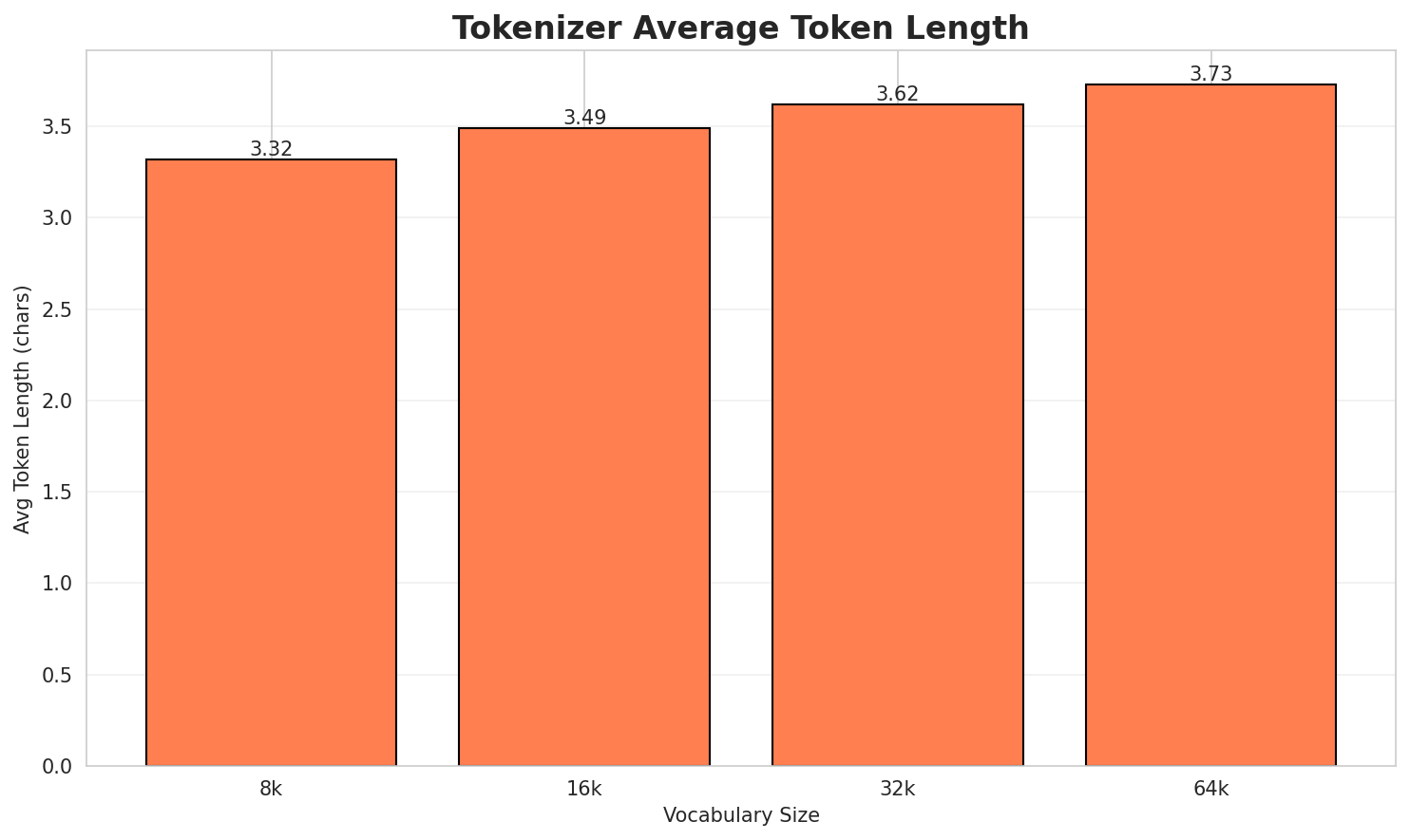
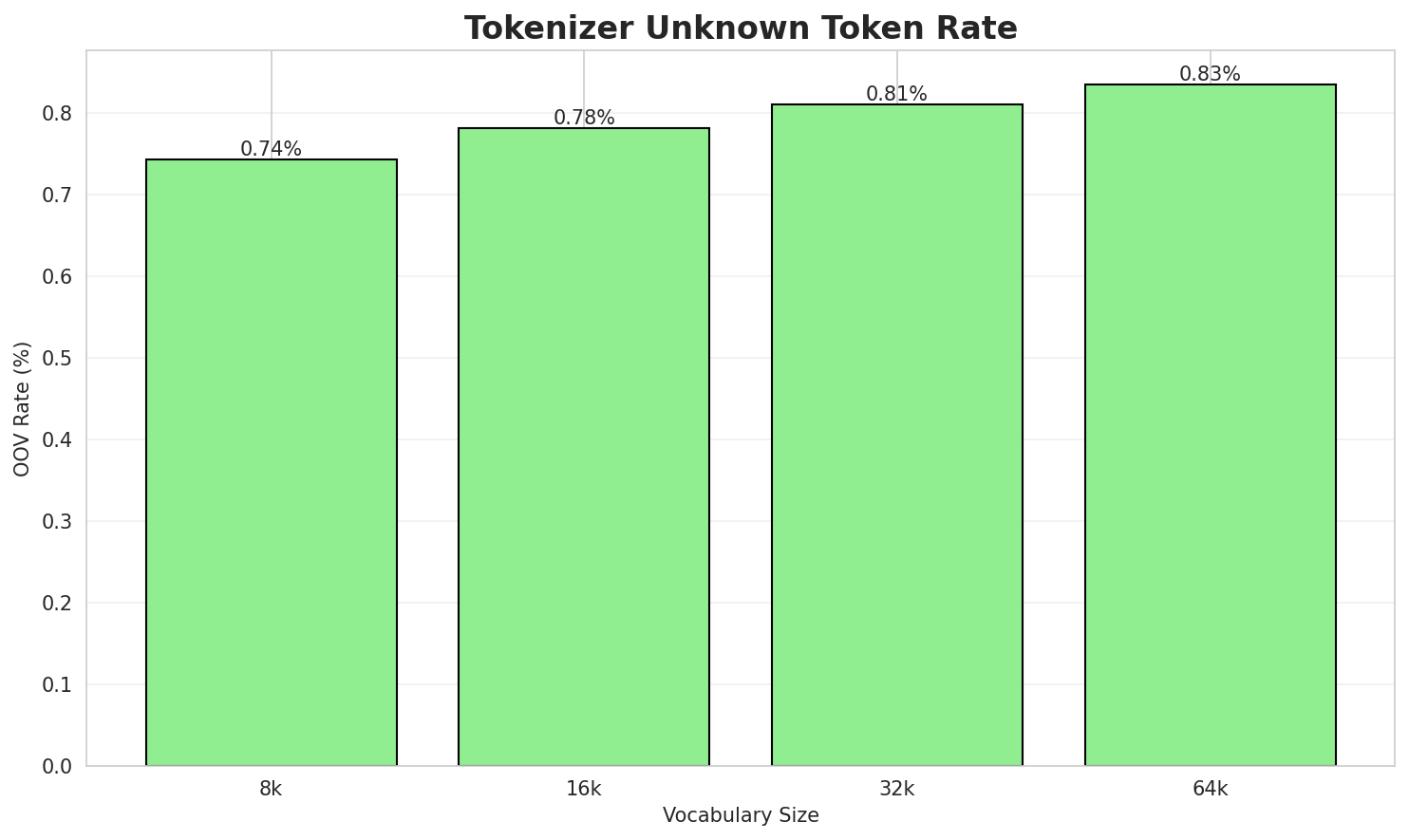
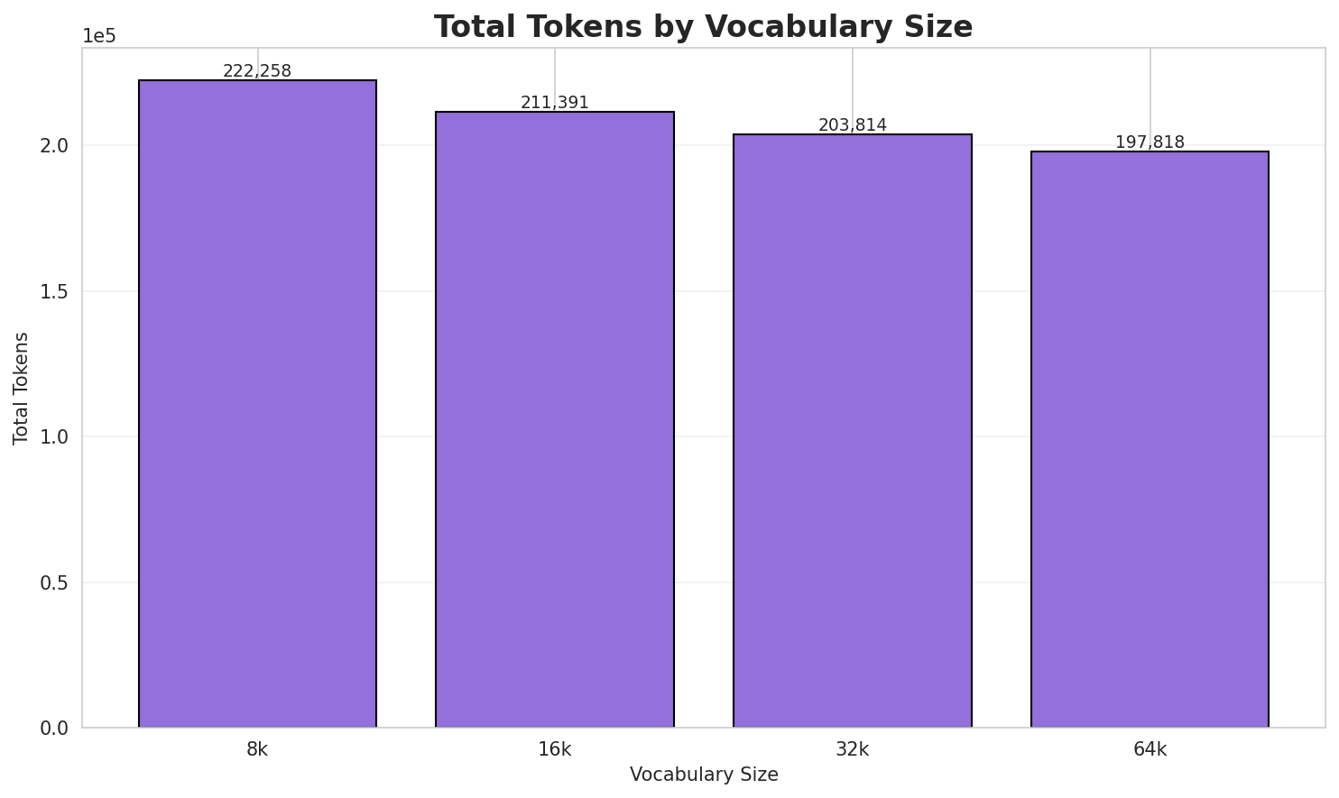
8k	3.313x	3.32	0.7428%	222,258
16k	3.483x	3.49	0.7810%	211,391
32k	3.612x	3.62	0.8101%	203,814
64k	3.722x 🏆	3.73	0.8346%	197,818

Tokenization Examples

Below are sample sentences tokenized with each vocabulary size:

Sample 1: Tółání Kʼish Chʼínítʼiʼ Tsé Chʼééchiiʼ yishtłizhii

Vocab	Tokens	Count
8k	▁tółání ▁k ʼ ish ▁ch ʼ ínít ʼ i ʼ ... (+7 more)	17
16k	▁tółání ▁k ʼ ish ▁ch ʼ ínít ʼ i ʼ ... (+6 more)	16
32k	▁tółání ▁k ʼ ish ▁ch ʼ ínít ʼ i ʼ ... (+6 more)	16
64k	▁tółání ▁k ʼ ish ▁ch ʼ ínít ʼ i ʼ ... (+6 more)	16

Sample 2: Naakaii Dootłʼizhii Bikéyahdę́ę́ʼ lókʼaatah naaʼahóóhai Tsiiʼyishbizhí Dineʼé Bi...

Vocab	Tokens	Count
8k	▁naakaii ▁dootł ʼ izhii ▁bikéyahdę́ę́ ʼ ▁lók ʼ aatah ▁naa ... (+16 more)	26
16k	▁naakaii ▁dootł ʼ izhii ▁bikéyahdę́ę́ ʼ ▁lók ʼ aatah ▁naa ... (+16 more)	26
32k	▁naakaii ▁dootł ʼ izhii ▁bikéyahdę́ę́ ʼ ▁lók ʼ aatah ▁naa ... (+16 more)	26
64k	▁naakaii ▁dootł ʼ izhii ▁bikéyahdę́ę́ ʼ ▁lók ʼ aatah ▁naa ... (+16 more)	26

Sample 3: Azeeʼ haajinítsoh Azeeʼ haajinítsʼóóz Azeeʼ haajiní łibáhígíí

Vocab	Tokens	Count
8k	▁azee ʼ ▁haajiní tsoh ▁azee ʼ ▁haajiní ts ʼ óóz ... (+4 more)	14
16k	▁azee ʼ ▁haajiní tsoh ▁azee ʼ ▁haajiní ts ʼ óóz ... (+4 more)	14
32k	▁azee ʼ ▁haajinítsoh ▁azee ʼ ▁haajiní ts ʼ óóz ▁azee ... (+3 more)	13
64k	▁azee ʼ ▁haajinítsoh ▁azee ʼ ▁haajiníts ʼ óóz ▁azee ʼ ... (+2 more)	12

Key Findings

• Best Compression: 64k achieves 3.722x compression
• Lowest UNK Rate: 8k with 0.7428% unknown tokens
• Trade-off: Larger vocabularies improve compression but increase model size
• Recommendation: 32k vocabulary provides optimal balance for production use

---

2. N-gram Model Evaluation

Results

N-gram	Variant	Perplexity	Entropy	Unique N-grams	Top-100 Coverage	Top-1000 Coverage
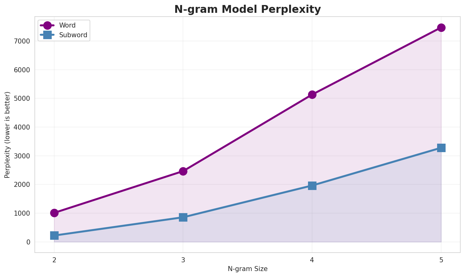
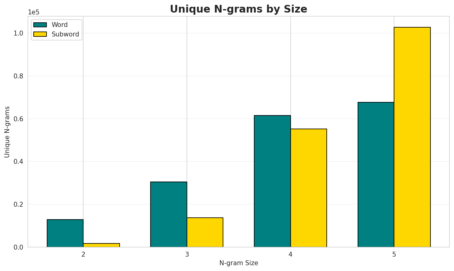
2-gram	Word	1,012	9.98	12,895	47.2%	81.9%
2-gram	Subword	222 🏆	7.79	1,668	72.2%	99.8%
3-gram	Word	2,466	11.27	30,460	36.6%	67.1%
3-gram	Subword	858	9.74	13,690	41.6%	89.2%
4-gram	Word	5,133	12.33	61,517	29.9%	56.5%
4-gram	Subword	1,964	10.94	55,169	29.2%	77.2%
5-gram	Word	7,471	12.87	67,722	25.5%	51.1%
5-gram	Subword	3,279	11.68	102,677	23.7%	69.1%

Top 5 N-grams by Size

2-grams (Word):

Rank	N-gram	Count
1	ndaʼałkaahí dóó	18,966
2	dóó ééʼdeetįįhii	18,949
3	ééʼdeetįįhii éí	18,878
4	áádóó éí	18,437
5	dah yikahjí	18,133

3-grams (Word):

Rank	N-gram	Count
1	ndaʼałkaahí dóó ééʼdeetįįhii	18,948
2	dóó ééʼdeetįįhii éí	18,878
3	dah yikahjí atah	18,128
4	ánoolinígíí dóó bichʼiyąʼ	16,794
5	dóó bichʼiyąʼ díí	16,604

4-grams (Word):

Rank	N-gram	Count
1	ndaʼałkaahí dóó ééʼdeetįįhii éí	18,877
2	ánoolinígíí dóó bichʼiyąʼ díí	16,603
3	dah yikahjí atah yisdzoh	15,997
4	atah yisdzoh áádóó éí	13,441
5	yikahjí atah yisdzoh áádóó	13,428

5-grams (Word):

Rank	N-gram	Count
1	dah yikahjí atah yisdzoh áádóó	13,428
2	yikahjí atah yisdzoh áádóó éí	13,421
3	hólǫ́ ndaʼałkaahí dóó ééʼdeetįįhii éí	13,312
4	deiłníigo dayózhí ánoolinígíí dóó bichʼiyąʼ	12,295
5	dayózhí ánoolinígíí dóó bichʼiyąʼ díí	12,263

2-grams (Subword):

Rank	N-gram	Count
1	í _	362,053
2	_ d	273,921
3	é í	184,110
4	_ é	173,881
5	_ b	173,418

3-grams (Subword):

Rank	N-gram	Count
1	é í _	182,329
2	_ b i	160,761
3	_ é í	154,684
4	ó ó _	132,006
5	d ó ó	123,733

4-grams (Subword):

Rank	N-gram	Count
1	_ é í _	154,592
2	d ó ó _	123,699
3	_ d ó ó	98,895
4	í g í í	52,301
5	g í í _	51,425

5-grams (Subword):

Rank	N-gram	Count
1	_ d ó ó _	98,891
2	í g í í _	51,394
3	í _ d ó ó	48,361
4	i _ é í _	38,726
5	d ó ó _ é	38,444

Key Findings

• Best Perplexity: 2-gram (subword) with 222
• Entropy Trend: Decreases with larger n-grams (more predictable)
• Coverage: Top-1000 patterns cover ~69% of corpus
• Recommendation: 4-gram or 5-gram for best predictive performance

---

3. Markov Chain Evaluation

Results

Context	Variant	Avg Entropy	Perplexity	Branching Factor	Unique Contexts	Predictability
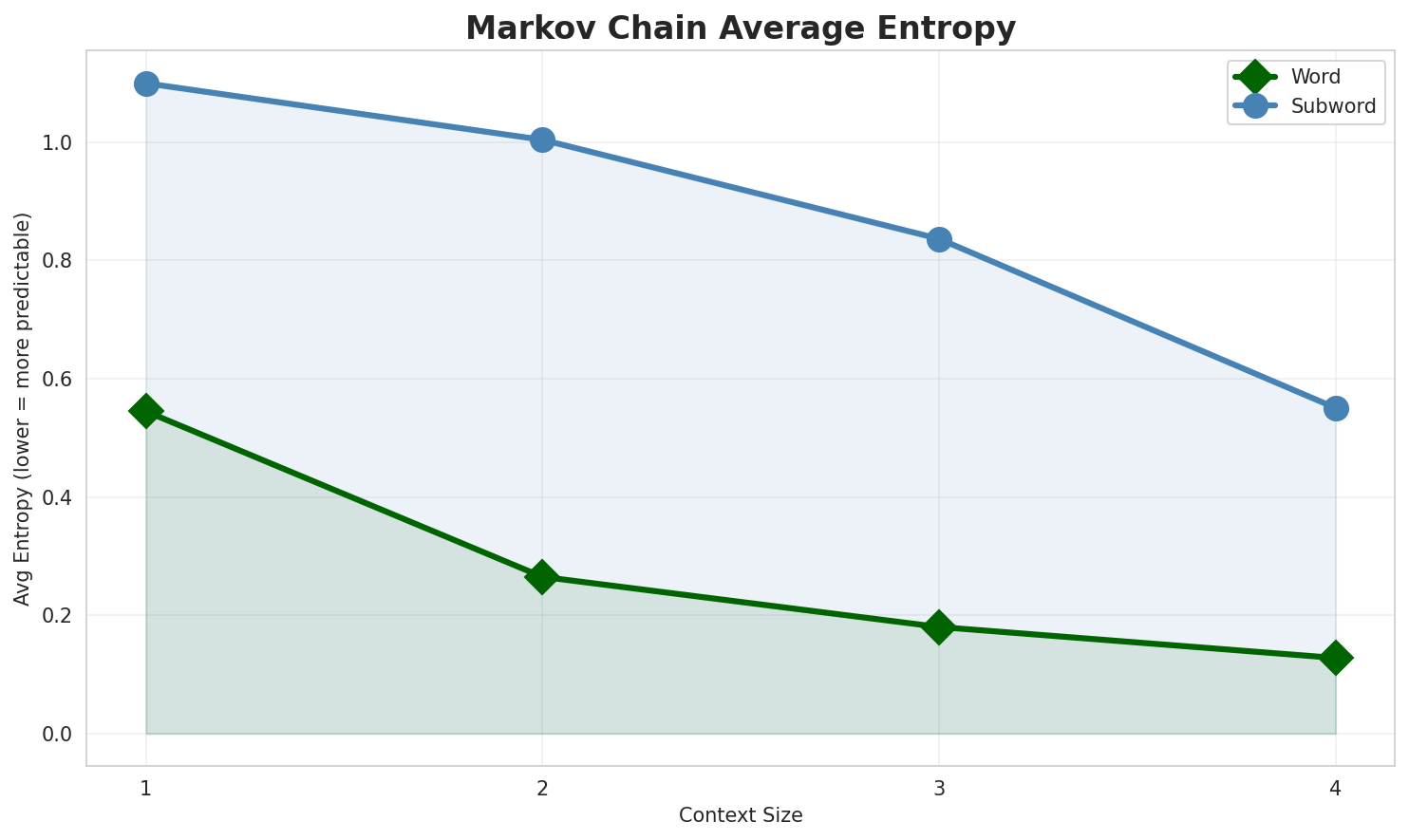
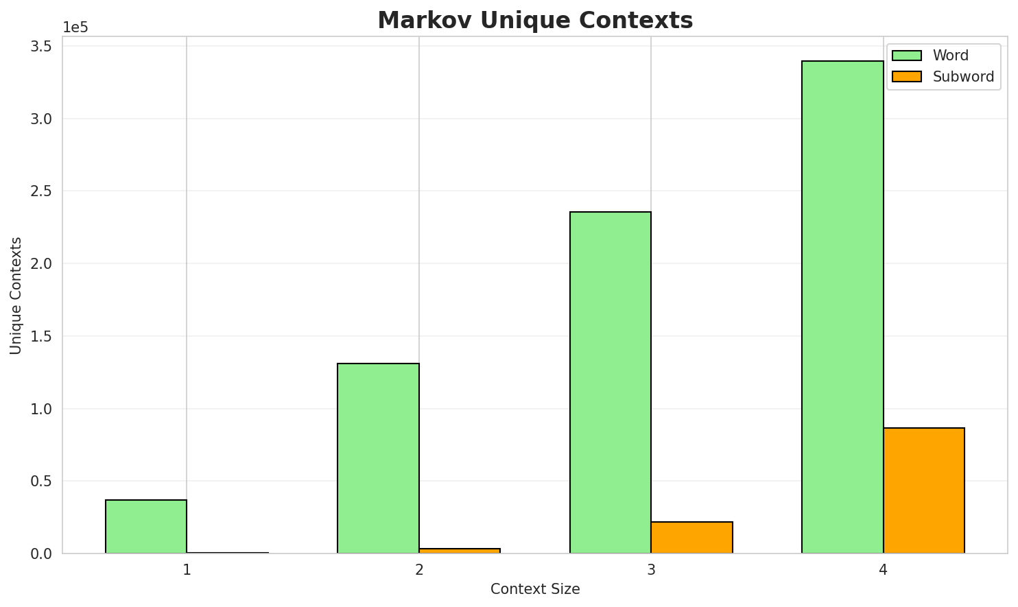
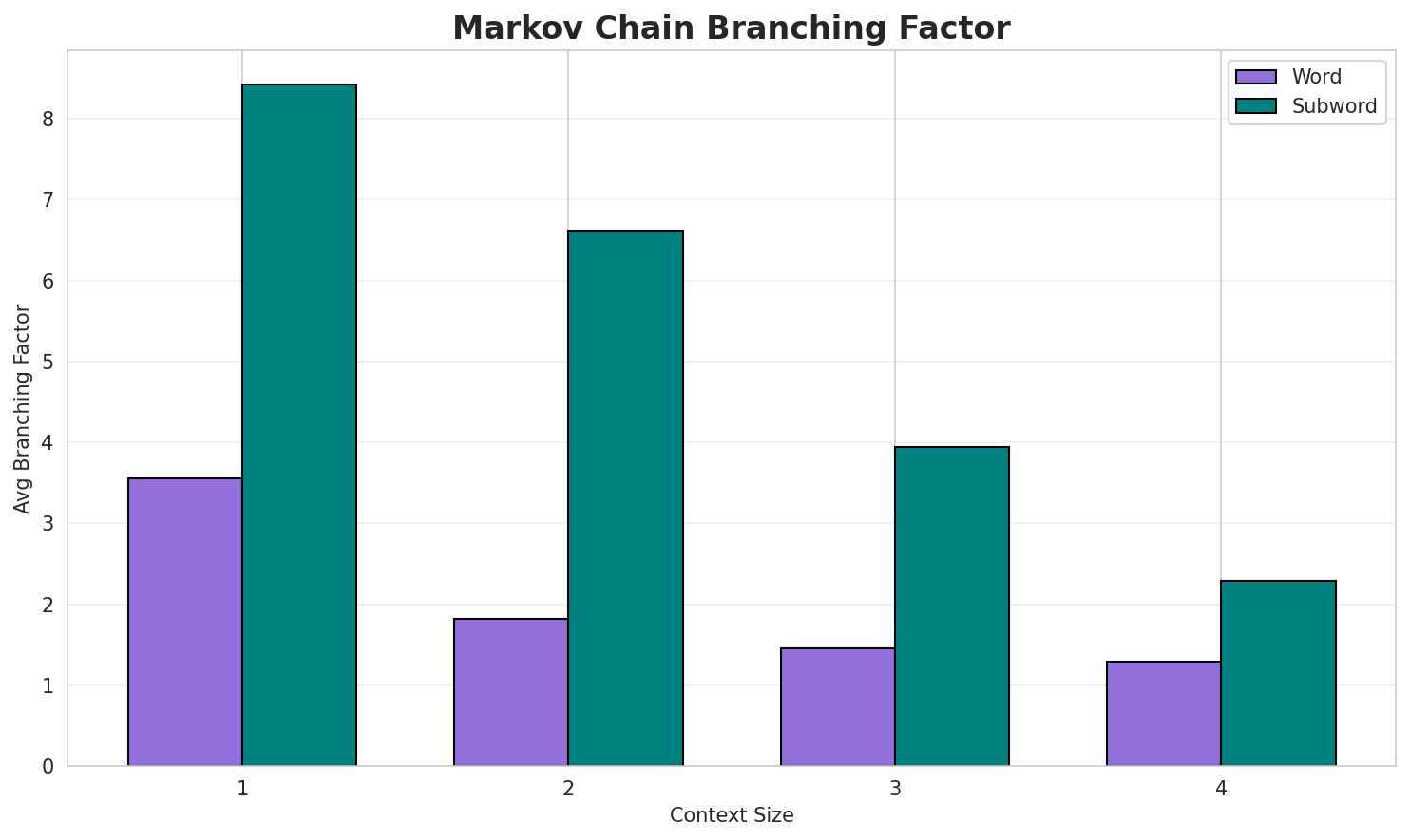
1	Word	0.5447	1.459	3.56	37,020	45.5%
1	Subword	1.0994	2.143	8.42	395	0.0%
2	Word	0.2649	1.202	1.82	130,895	73.5%
2	Subword	1.0039	2.005	6.61	3,325	0.0%
3	Word	0.1801	1.133	1.46	235,498	82.0%
3	Subword	0.8364	1.786	3.94	21,977	16.4%
4	Word	0.1277 🏆	1.093	1.29	339,354	87.2%
4	Subword	0.5506	1.465	2.29	86,495	44.9%

Generated Text Samples (Word-based)

Below are text samples generated from each word-based Markov chain model:

Context Size 1:

1. éí łigai baʼáádígíí éí kéyah dah ndaaʼeełí łánídę́ę́ʼ tłʼiish dah yikahjí atah yisdzoh áádóó éí chʼi...
2. dóó chʼał dootłʼizhí bikédaayahdi tʼéiyá hólǫ́ ndaʼałkaahí dóó ééʼdeetįįhii éí diłhił shádiʼááh dóó ...
3. dah daalgai bitsiitsʼiin éí nahasdzáán tʼáá díkwíí mm áníłtso bitsʼíís éí yótʼáahdi tsídii tsídígíí ...

Context Size 2:

1. ndaʼałkaahí dóó ééʼdeetįįhii éí certhilauda benguelensis deiłníigo dayózhí ánoolinígíí dóó bichʼiyąʼ...
2. dóó ééʼdeetįįhii éí euscarthmus rufomarginatus deiłníigo dayózhí ánoolinígíí dóó bichʼiyąʼ díí naʼas...
3. ééʼdeetįįhii éí rhamphiophis oxyrhynchus deiłníigo dayózhí ánoolinígíí dóó bichʼiyąʼ díí tsídii biką...

Context Size 3:

1. ndaʼałkaahí dóó ééʼdeetįįhii éí dendropsophus koechlini deiłníigo dayózhí ánoolinígíí dóó bichʼiyąʼ ...
2. dóó ééʼdeetįįhii éí ptilopsis leucotis deiłníigo dayózhí ánoolinígíí dóó bichʼiyąʼ díí tłʼiish éí 30...
3. dah yikahjí atah yisdzoh áádóó éí naakaii łizhiní bikéyahdi hólǫ́ ndaʼałkaahí dóó ééʼdeetįįhii éí xe...

Context Size 4:

1. ndaʼałkaahí dóó ééʼdeetįįhii éí dendrolagus deiłníigo deiyózhí díí nahatʼeʼiitsoh éí 17 ałʼąą ádaatʼ...
2. ánoolinígíí dóó bichʼiyąʼ díí naʼashǫ́ʼii éí 4 5di asdzoh áníłtso bitsʼíís éí chʼilgo dootłʼizh bits...
3. dah yikahjí atah yisdzoh áádóó éí magí bitseeʼ noodǫ́zí bikéyahdi tʼéiyá hólǫ́ ndaʼałkaahí dóó ééʼde...

Generated Text Samples (Subword-based)

Below are text samples generated from each subword-based Markov chain model:

Context Size 1:

1. _béíígaiy_"_yaʼ_
2. i_yąʼééí_ttą́._ée
3. í_éí_éí_tsh_áááʼ

Context Size 2:

1. í_dóó_atahdę́ę́ʼ_yę́
2. _dóó_bináhooly_oo
3. éí_bitoʼ_atah_yik

Context Size 3:

1. éí_naaʼałkaahí_éí_
2. _bitłʼaahjí_kélchí
3. _éí_naaznilzhin;_b

Context Size 4:

1. _éí_naashchʼąąʼ_éí_
2. dóó_éí_hólǫ́._ndaʼał
3. _dóó_ééʼdeetįįhii_é

Key Findings

• Best Predictability: Context-4 (word) with 87.2% predictability
• Branching Factor: Decreases with context size (more deterministic)
• Memory Trade-off: Larger contexts require more storage (86,495 contexts)
• Recommendation: Context-3 or Context-4 for text generation

---

4. Vocabulary Analysis

Statistics

Metric	Value
Vocabulary Size	15,109
Total Tokens	1,314,110
Mean Frequency	86.98
Median Frequency	4
Frequency Std Dev	1812.30

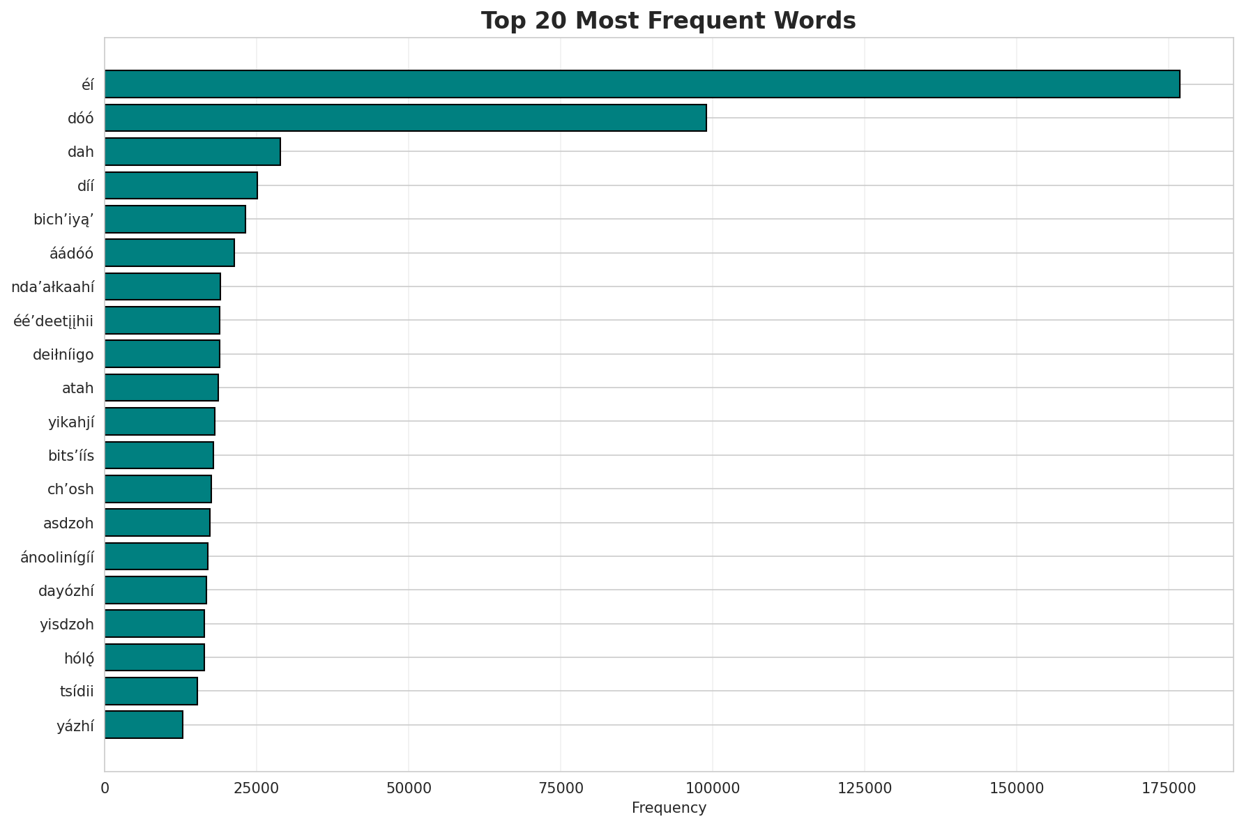
Most Common Words

Rank	Word	Frequency
1	éí	176,805
2	dóó	99,009
3	dah	28,837
4	díí	25,092
5	bichʼiyąʼ	23,153
6	áádóó	21,278
7	ndaʼałkaahí	19,035
8	ééʼdeetįįhii	18,949
9	deiłníigo	18,893
10	atah	18,728

Least Common Words (from vocabulary)

Rank	Word	Frequency
1	milano	2
2	príncipe	2
3	butiama	2
4	àɖokun	2
5	yí	2
6	azɔ	2
7	àkpɔ̀	2
8	gbɔ̀	2
9	panafrikan	2
10	modèle	2

Zipf's Law Analysis

Metric	Value
Zipf Coefficient	1.3602
R² (Goodness of Fit)	0.987051
Adherence Quality	excellent

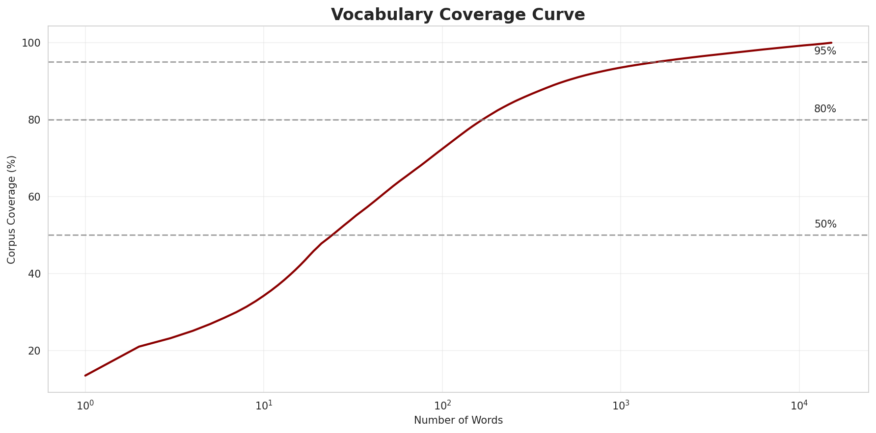
Coverage Analysis

Top N Words	Coverage
Top 100	72.4%
Top 1,000	93.5%
Top 5,000	97.8%
Top 10,000	99.2%

Key Findings

• Zipf Compliance: R²=0.9871 indicates excellent adherence to Zipf's law
• High Frequency Dominance: Top 100 words cover 72.4% of corpus
• Long Tail: 5,109 words needed for remaining 0.8% coverage

---

5. Word Embeddings Evaluation

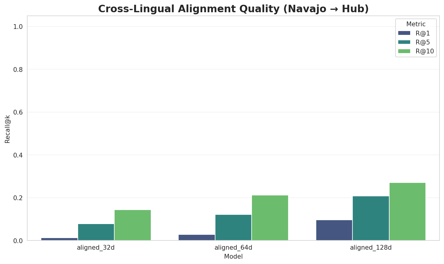
5.1 Cross-Lingual Alignment

5.2 Model Comparison

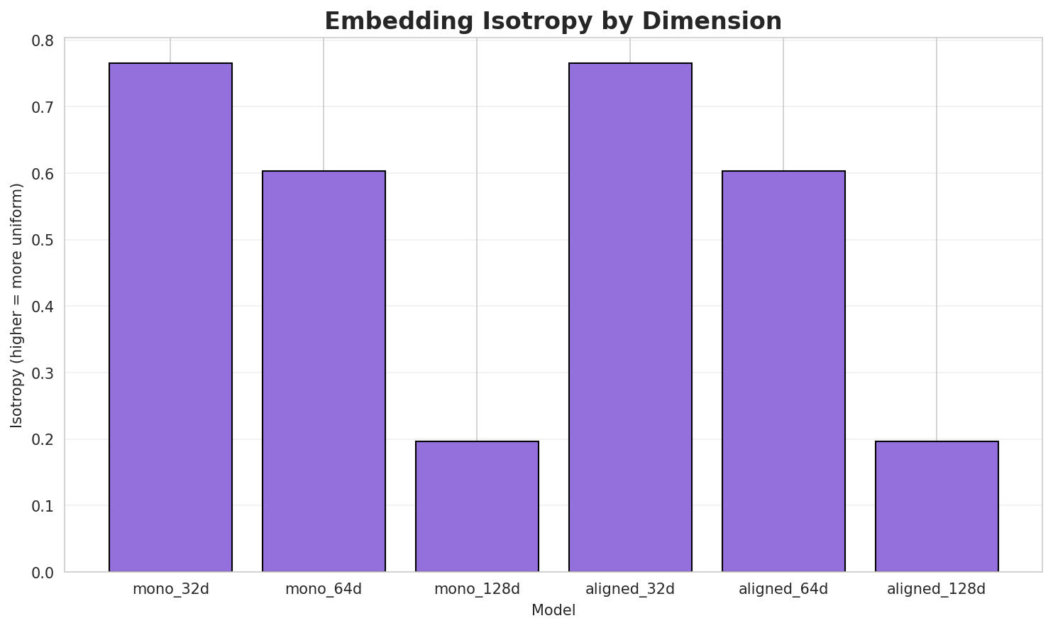
Model	Dimension	Isotropy	Semantic Density	Alignment R@1	Alignment R@10
mono_32d	32	0.7658 🏆	0.3405	N/A	N/A
mono_64d	64	0.6030	0.2817	N/A	N/A
mono_128d	128	0.1964	0.2867	N/A	N/A
aligned_32d	32	0.7658	0.3269	0.0120	0.1440
aligned_64d	64	0.6030	0.2833	0.0280	0.2120
aligned_128d	128	0.1964	0.2859	0.0960	0.2700

Key Findings

• Best Isotropy: mono_32d with 0.7658 (more uniform distribution)
• Semantic Density: Average pairwise similarity of 0.3008. Lower values indicate better semantic separation.
• Alignment Quality: Aligned models achieve up to 9.6% R@1 in cross-lingual retrieval.
• Recommendation: 128d aligned for best cross-lingual performance

---

6. Morphological Analysis (Experimental)

This section presents an automated morphological analysis derived from the statistical divergence between word-level and subword-level models. By analyzing where subword predictability spikes and where word-level coverage fails, we can infer linguistic structures without supervised data.

6.1 Productivity & Complexity

Metric	Value	Interpretation	Recommendation
Productivity Index	5.000	High morphological productivity	Reliable analysis
Idiomaticity Gap	-0.261	Low formulaic content	-

6.2 Affix Inventory (Productive Units)

These are the most productive prefixes and suffixes identified by sampling the vocabulary for global substitutability patterns. A unit is considered an affix if stripping it leaves a valid stem that appears in other contexts.

Productive Prefixes

Prefix	Examples
-a	allotment, amá, apodora
-bi	bikʼa, bichʼoshtsoh, bitsʼáozʼaʼ
-d	diastema, dryocalamus, deezlíníidi
-b	bílátaʼiitsóóh, bikʼa, bí
-t	tséhaagééd, tóńlį́, tʼiistsooítah
-s	sylvilagus, sturnira, sturnus
-n	natalobatrachus, neomixis, nahonitłʼahii
-c	certhiaxis, chʼiltaalzhahii, chʼahí

Productive Suffixes

Suffix	Examples
-s	himalayensis, sylvilagus, femoralis
-us	sylvilagus, dryocalamus, sturnus
-í	wálázhiní, bí, magítʼą́ʼí
-i	tséʼałnáoztʼiʼíidi, deezlíníidi, chʼiltaalzhahii
-a	sturnira, fuscicauda, bikʼa
-is	himalayensis, femoralis, ichthyophis
-ii	chʼiltaalzhahii, dáághahii, nahonitłʼahii
-íí	yeeyáʼdaałtíʼígíí, díkiwíí, dadijoolígíí

6.3 Bound Stems (Lexical Roots)

Bound stems are high-frequency subword units that are semantically cohesive but rarely appear as standalone words. These often correspond to the 'core' of a word that requires inflection or derivation to be valid.

Stem	Cohesion	Substitutability	Examples
ikah	2.28x	8 contexts	yikahí, yikahji, yikahjí
itsʼ	1.33x	31 contexts	bitsʼáh, bitsʼoh, ditsʼoz
tsʼí	1.63x	14 contexts	tsʼídá, tsʼííh, tsʼímah
éyah	1.67x	13 contexts	kéyah, kéyahdi, hakéyah
iłní	1.98x	8 contexts	deiłní, nihiłní, ádeiłní
sʼíí	1.87x	9 contexts	tsʼííh, bitsʼíí, atsʼíís
yika	2.28x	5 contexts	yikał, yikahí, yikahji
kahj	2.28x	5 contexts	yikahji, yikahjí, daakahjí
kéya	1.67x	9 contexts	kéyah, kéyahdi, hakéyah
níig	1.81x	7 contexts	níigo, aníigo, aaníigo
iníg	2.05x	5 contexts	kinígíí, ádinígíí, nízinígíí
bich	1.44x	11 contexts	bichʼįʼ, bichąąʼ, bichʼil

6.4 Affix Compatibility (Co-occurrence)

This table shows which prefixes and suffixes most frequently co-occur on the same stems, revealing the 'stacking' rules of the language's morphology.

Prefix	Suffix	Frequency	Examples
-c	-s	249 words	chrysops, clematis
-p	-s	243 words	platymantis, parvirostris
-d	-í	213 words	dinilbáhí, dziłghą́ʼí
-a	-s	184 words	arvalis, antrozous
-n	-í	184 words	naalzheehígíí, naʼazísí
-s	-s	156 words	sclerurus, scytodes
-p	-us	138 words	perspicillatus, pteruthius
-c	-us	131 words	castaneus, chroicocephalus
-c	-a	126 words	crocata, cyanoleuca
-t	-í	123 words	tłʼohtsʼózí, tłʼohwaaʼí

6.5 Recursive Morpheme Segmentation

Using Recursive Hierarchical Substitutability, we decompose complex words into their constituent morphemes. This approach handles nested affixes (e.g., prefix-prefix-root-suffix).

Word	Suggested Split	Confidence	Stem
daʼałhosh	daʼałho-s-h	7.5	s
moluccensis	moluccen-s-is	7.5	s
daatsʼísí	daatsʼí-s-í	7.5	s
sminthopsis	sminthop-s-is	7.5	s
barbadensis	barbaden-s-is	7.5	s
chʼoshtsoh	chʼosht-s-oh	7.5	s
leucopsis	leucop-s-is	7.5	s
pretiosus	pretio-s-us	7.5	s
dlǫ́ʼiitsoh	dlǫ́ʼiit-s-oh	7.5	s
dinilzhinhgo	dinilzhin-h-go	7.5	h
mąʼiikʼǫsh	mąʼiikʼǫ-s-h	7.5	s
portoricensis	portoricen-s-is	7.5	s
natalensis	natalen-s-is	7.5	s
yildeełítsoh	yildeełít-s-oh	7.5	s
iichʼąhiitsʼósí	iichʼąhiitsʼó-s-í	7.5	s

6.6 Linguistic Interpretation

Automated Insight: The language Navajo shows high morphological productivity. The subword models are significantly more efficient than word models, suggesting a rich system of affixation or compounding.

---

7. Summary & Recommendations

Production Recommendations

Component	Recommended	Rationale
Tokenizer	64k BPE	Best compression (3.72x)
N-gram	2-gram	Lowest perplexity (222)
Markov	Context-4	Highest predictability (87.2%)
Embeddings	100d	Balanced semantic capture and isotropy

---

Appendix: Metrics Glossary & Interpretation Guide

This section provides definitions, intuitions, and guidance for interpreting the metrics used throughout this report.

Tokenizer Metrics

Compression Ratio

Definition: The ratio of characters to tokens (chars/token). Measures how efficiently the tokenizer represents text.

Intuition: Higher compression means fewer tokens needed to represent the same text, reducing sequence lengths for downstream models. A 3x compression means ~3 characters per token on average.

What to seek: Higher is generally better for efficiency, but extremely high compression may indicate overly aggressive merging that loses morphological information.

Average Token Length (Fertility)

Definition: Mean number of characters per token produced by the tokenizer.

Intuition: Reflects the granularity of tokenization. Longer tokens capture more context but may struggle with rare words; shorter tokens are more flexible but increase sequence length.

What to seek: Balance between 2-5 characters for most languages. Arabic/morphologically-rich languages may benefit from slightly longer tokens.

Unknown Token Rate (OOV Rate)

Definition: Percentage of tokens that map to the unknown/UNK token, indicating words the tokenizer cannot represent.

Intuition: Lower OOV means better vocabulary coverage. High OOV indicates the tokenizer encounters many unseen character sequences.

What to seek: Below 1% is excellent; below 5% is acceptable. BPE tokenizers typically achieve very low OOV due to subword fallback.

N-gram Model Metrics

Perplexity

Definition: Measures how "surprised" the model is by test data. Mathematically: 2^(cross-entropy). Lower values indicate better prediction.

Intuition: If perplexity is 100, the model is as uncertain as if choosing uniformly among 100 options at each step. A perplexity of 10 means effectively choosing among 10 equally likely options.

What to seek: Lower is better. Perplexity decreases with larger n-grams (more context). Values vary widely by language and corpus size.

Entropy

Definition: Average information content (in bits) needed to encode the next token given the context. Related to perplexity: perplexity = 2^entropy.

Intuition: High entropy means high uncertainty/randomness; low entropy means predictable patterns. Natural language typically has entropy between 1-4 bits per character.

What to seek: Lower entropy indicates more predictable text patterns. Entropy should decrease as n-gram size increases.

Coverage (Top-K)

Definition: Percentage of corpus occurrences explained by the top K most frequent n-grams.

Intuition: High coverage with few patterns indicates repetitive/formulaic text; low coverage suggests diverse vocabulary usage.

What to seek: Depends on use case. For language modeling, moderate coverage (40-60% with top-1000) is typical for natural text.

Markov Chain Metrics

Average Entropy

Definition: Mean entropy across all contexts, measuring average uncertainty in next-word prediction.

Intuition: Lower entropy means the model is more confident about what comes next. Context-1 has high entropy (many possible next words); Context-4 has low entropy (few likely continuations).

What to seek: Decreasing entropy with larger context sizes. Very low entropy (<0.1) indicates highly deterministic transitions.

Branching Factor

Definition: Average number of unique next tokens observed for each context.

Intuition: High branching = many possible continuations (flexible but uncertain); low branching = few options (predictable but potentially repetitive).

What to seek: Branching factor should decrease with context size. Values near 1.0 indicate nearly deterministic chains.

Predictability

Definition: Derived metric: (1 - normalized_entropy) × 100%. Indicates how deterministic the model's predictions are.

Intuition: 100% predictability means the next word is always certain; 0% means completely random. Real text falls between these extremes.

What to seek: Higher predictability for text generation quality, but too high (>98%) may produce repetitive output.

Vocabulary & Zipf's Law Metrics

Zipf's Coefficient

Definition: The slope of the log-log plot of word frequency vs. rank. Zipf's law predicts this should be approximately -1.

Intuition: A coefficient near -1 indicates the corpus follows natural language patterns where a few words are very common and most words are rare.

What to seek: Values between -0.8 and -1.2 indicate healthy natural language distribution. Deviations may suggest domain-specific or artificial text.

R² (Coefficient of Determination)

Definition: Measures how well the linear fit explains the frequency-rank relationship. Ranges from 0 to 1.

Intuition: R² near 1.0 means the data closely follows Zipf's law; lower values indicate deviation from expected word frequency patterns.

What to seek: R² > 0.95 is excellent; > 0.99 indicates near-perfect Zipf adherence typical of large natural corpora.

Vocabulary Coverage

Definition: Cumulative percentage of corpus tokens accounted for by the top N words.

Intuition: Shows how concentrated word usage is. If top-100 words cover 50% of text, the corpus relies heavily on common words.

What to seek: Top-100 covering 30-50% is typical. Higher coverage indicates more repetitive text; lower suggests richer vocabulary.

Word Embedding Metrics

Isotropy

Definition: Measures how uniformly distributed vectors are in the embedding space. Computed as the ratio of minimum to maximum singular values.

Intuition: High isotropy (near 1.0) means vectors spread evenly in all directions; low isotropy means vectors cluster in certain directions, reducing expressiveness.

What to seek: Higher isotropy generally indicates better-quality embeddings. Values > 0.1 are reasonable; > 0.3 is good. Lower-dimensional embeddings tend to have higher isotropy.

Average Norm

Definition: Mean magnitude (L2 norm) of word vectors in the embedding space.

Intuition: Indicates the typical "length" of vectors. Consistent norms suggest stable training; high variance may indicate some words are undertrained.

What to seek: Relatively consistent norms across models. The absolute value matters less than consistency (low std deviation).

Cosine Similarity

Definition: Measures angular similarity between vectors, ranging from -1 (opposite) to 1 (identical direction).

Intuition: Words with similar meanings should have high cosine similarity. This is the standard metric for semantic relatedness in embeddings.

What to seek: Semantically related words should score > 0.5; unrelated words should be near 0. Synonyms often score > 0.7.

t-SNE Visualization

Definition: t-Distributed Stochastic Neighbor Embedding - a dimensionality reduction technique that preserves local structure for visualization.

Intuition: Clusters in t-SNE plots indicate groups of semantically related words. Spread indicates vocabulary diversity; tight clusters suggest semantic coherence.

What to seek: Meaningful clusters (e.g., numbers together, verbs together). Avoid over-interpreting distances - t-SNE preserves local, not global, structure.

General Interpretation Guidelines

1. Compare within model families: Metrics are most meaningful when comparing models of the same type (e.g., 8k vs 64k tokenizer).
2. Consider trade-offs: Better performance on one metric often comes at the cost of another (e.g., compression vs. OOV rate).
3. Context matters: Optimal values depend on downstream tasks. Text generation may prioritize different metrics than classification.
4. Corpus influence: All metrics are influenced by corpus characteristics. Wikipedia text differs from social media or literature.
5. Language-specific patterns: Morphologically rich languages (like Arabic) may show different optimal ranges than analytic languages.

Visualizations Index

Visualization	Description
Tokenizer Compression	Compression ratios by vocabulary size
Tokenizer Fertility	Average token length by vocabulary
Tokenizer OOV	Unknown token rates
Tokenizer Total Tokens	Total tokens by vocabulary
N-gram Perplexity	Perplexity by n-gram size
N-gram Entropy	Entropy by n-gram size
N-gram Coverage	Top pattern coverage
N-gram Unique	Unique n-gram counts
Markov Entropy	Entropy by context size
Markov Branching	Branching factor by context
Markov Contexts	Unique context counts
Zipf's Law	Frequency-rank distribution with fit
Vocab Frequency	Word frequency distribution
Top 20 Words	Most frequent words
Vocab Coverage	Cumulative coverage curve
Embedding Isotropy	Vector space uniformity
Embedding Norms	Vector magnitude distribution
Embedding Similarity	Word similarity heatmap
Nearest Neighbors	Similar words for key terms
t-SNE Words	2D word embedding visualization
t-SNE Sentences	2D sentence embedding visualization
Position Encoding	Encoding method comparison
Model Sizes	Storage requirements
Performance Dashboard	Comprehensive performance overview

---

About This Project

Data Source

Models trained on wikipedia-monthly - a monthly snapshot of Wikipedia articles across 300+ languages.

Project

A project by Wikilangs - Open-source NLP models for every Wikipedia language.

Maintainer

Omar Kamali - Omneity Labs

Citation

If you use these models in your research, please cite:

@misc{wikilangs2025,
  author = {Kamali, Omar},
  title = {Wikilangs: Open NLP Models for Wikipedia Languages},
  year = {2025},
  doi = {10.5281/zenodo.18073153},
  publisher = {Zenodo},
  url = {https://huggingface.co/wikilangs}
  institution = {Omneity Labs}
}

License

MIT License - Free for academic and commercial use.

Links

• 🌐 Website: wikilangs.org
• 🤗 Models: huggingface.co/wikilangs
• 📊 Data: wikipedia-monthly
• 👤 Author: Omar Kamali
• 🤝 Sponsor: Featherless AI

---

Generated by Wikilangs Models Pipeline

Report Date: 2026-01-10 16:24:15