README.md

metadata

language: zgh
language_name: Standard Moroccan Tamazight
language_family: berber
tags:
  - wikilangs
  - nlp
  - tokenizer
  - embeddings
  - n-gram
  - markov
  - wikipedia
  - feature-extraction
  - sentence-similarity
  - tokenization
  - n-grams
  - markov-chain
  - text-mining
  - fasttext
  - babelvec
  - vocabulous
  - vocabulary
  - monolingual
  - family-berber
license: mit
library_name: wikilangs
pipeline_tag: text-generation
datasets:
  - omarkamali/wikipedia-monthly
dataset_info:
  name: wikipedia-monthly
  description: Monthly snapshots of Wikipedia articles across 300+ languages
metrics:
  - name: best_compression_ratio
    type: compression
    value: 3.844
  - name: best_isotropy
    type: isotropy
    value: 0.7259
  - name: vocabulary_size
    type: vocab
    value: 0
generated: 2026-01-11T00:00:00.000Z

Standard Moroccan Tamazight - Wikilangs Models

Comprehensive Research Report & Full Ablation Study

This repository contains NLP models trained and evaluated by Wikilangs, specifically on Standard Moroccan Tamazight Wikipedia data. We analyze tokenizers, n-gram models, Markov chains, vocabulary statistics, and word embeddings.

📋 Repository Contents

Models & Assets

• Tokenizers (8k, 16k, 32k, 64k)
• N-gram models (2, 3, 4, 5-gram)
• Markov chains (context of 1, 2, 3, 4 and 5)
• Subword N-gram and Markov chains
• Embeddings in various sizes and dimensions (aligned and unaligned)
• Language Vocabulary
• Language Statistics

Analysis and Evaluation

• 1. Tokenizer Evaluation
• 2. N-gram Model Evaluation
• 3. Markov Chain Evaluation
• 4. Vocabulary Analysis
• 5. Word Embeddings Evaluation
• 6. Morphological Analysis (Experimental)
• 7. Summary & Recommendations
• Metrics Glossary
• Visualizations Index

---

1. Tokenizer Evaluation

Results

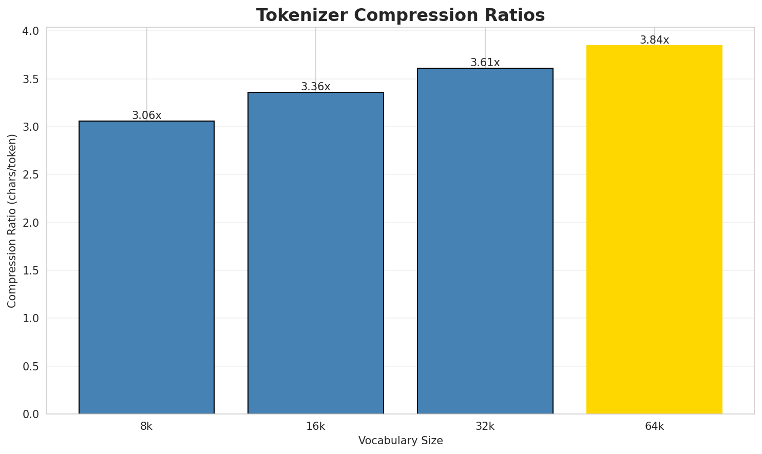
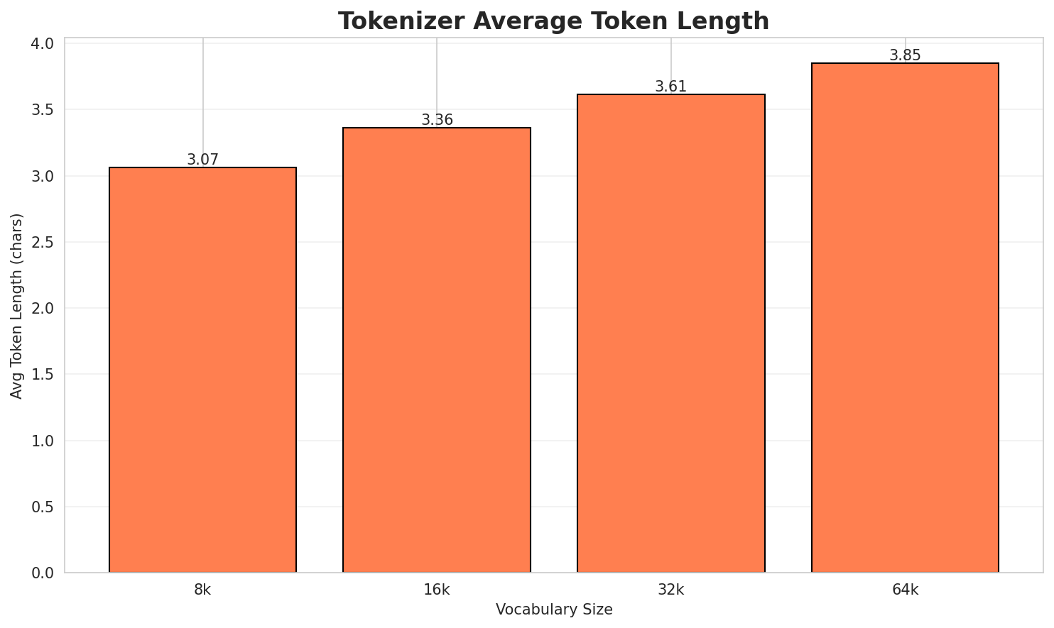
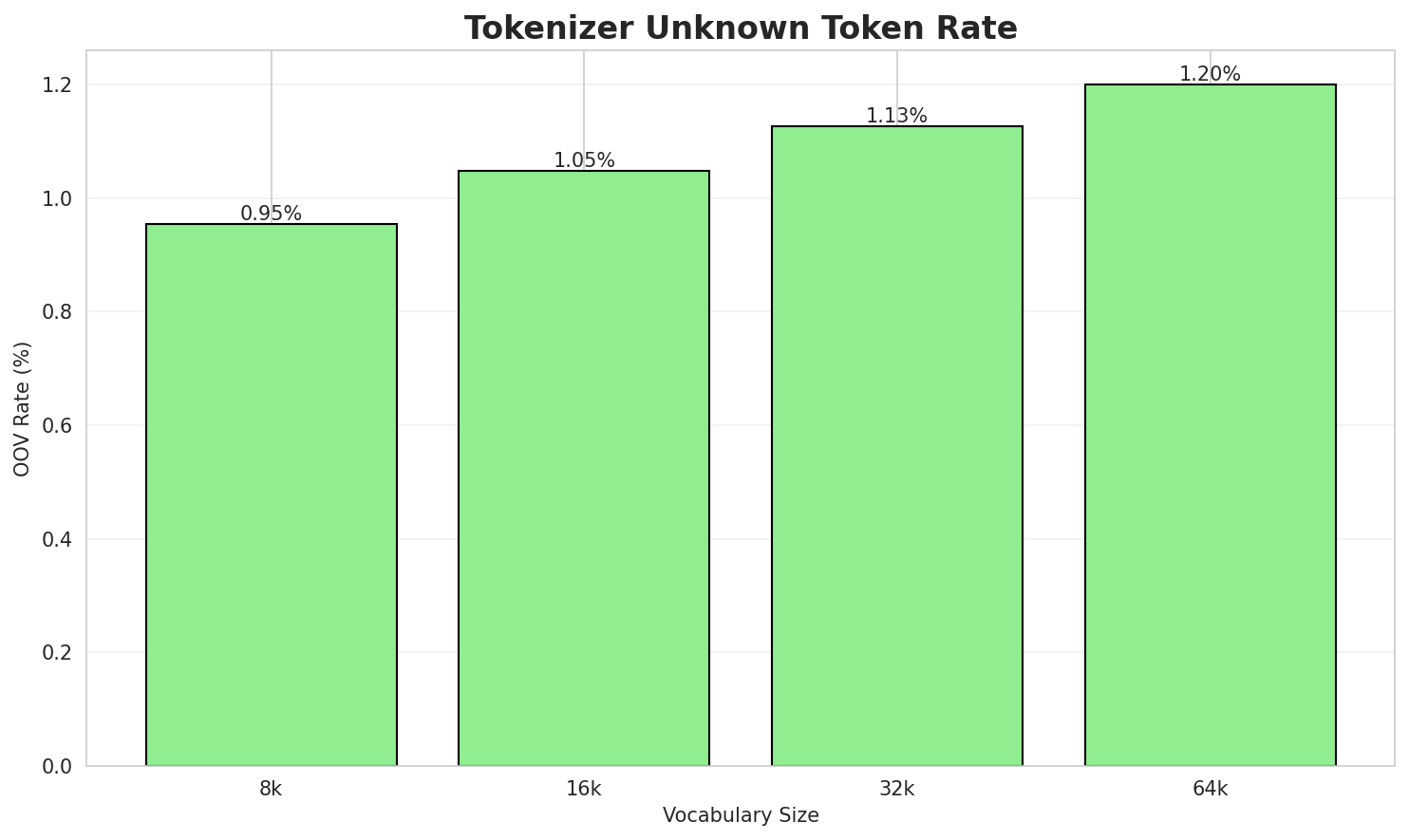
Vocab Size	Compression	Avg Token Len	UNK Rate	Total Tokens
8k	3.062x	3.07	0.9549%	377,124
16k	3.360x	3.36	1.0478%	343,658
32k	3.609x	3.61	1.1257%	319,893
64k	3.844x 🏆	3.85	1.1990%	300,327

Tokenization Examples

Below are sample sentences tokenized with each vocabulary size:

Sample 1: thumb ⴱⵉ ⴱⵉ ⵙⵉ ⵏⵖ BBC (ⵙ ⵜⵏⴳⵍⵉⵣⵜ: British Broadcasting Corporation) ⵉⵙⴰⵖⵓⵍⵏ

Vocab	Tokens	Count
8k	▁thumb ▁ⴱⵉ ▁ⴱⵉ ▁ⵙⵉ ▁ⵏⵖ ▁b bc ▁( ⵙ ▁ⵜⵏⴳⵍⵉⵣⵜ ... (+16 more)	26
16k	▁thumb ▁ⴱⵉ ▁ⴱⵉ ▁ⵙⵉ ▁ⵏⵖ ▁bbc ▁( ⵙ ▁ⵜⵏⴳⵍⵉⵣⵜ : ... (+9 more)	19
32k	▁thumb ▁ⴱⵉ ▁ⴱⵉ ▁ⵙⵉ ▁ⵏⵖ ▁bbc ▁( ⵙ ▁ⵜⵏⴳⵍⵉⵣⵜ : ... (+8 more)	18
64k	▁thumb ▁ⴱⵉ ▁ⴱⵉ ▁ⵙⵉ ▁ⵏⵖ ▁bbc ▁( ⵙ ▁ⵜⵏⴳⵍⵉⵣⵜ : ... (+5 more)	15

Sample 2: ⴰⴳⴰⴷⴰⵣ ⴰⴼⵕⴰⵏⵚⵉⵚ ⵉⴳⴰ ⴰⴳⴷⵓⵣ ⴷ ⴰⵙⴷⴷⵉ ⵏ ⵡⴰⵙⵖⵏⵣⵉ ⴳ ⵜⴰⴷⴷⵓⵔⵜ ⵜⴰⴼⵕⴰⵏⵚⵉⵚⵜ, ⵏ ⵓⵔⵍⵢⴰⵏⵣ ⴰⵎⴰⵢ...

Vocab	Tokens	Count
8k	▁ⴰⴳⴰ ⴷⴰⵣ ▁ⴰⴼⵕⴰⵏⵚⵉⵚ ▁ⵉⴳⴰ ▁ⴰⴳⴷ ⵓⵣ ▁ⴷ ▁ⴰⵙⴷⴷⵉ ▁ⵏ ▁ⵡⴰⵙ ... (+19 more)	29
16k	▁ⴰⴳⴰⴷⴰⵣ ▁ⴰⴼⵕⴰⵏⵚⵉⵚ ▁ⵉⴳⴰ ▁ⴰⴳⴷ ⵓⵣ ▁ⴷ ▁ⴰⵙⴷⴷⵉ ▁ⵏ ▁ⵡⴰⵙ ⵖⵏⵣⵉ ... (+17 more)	27
32k	▁ⴰⴳⴰⴷⴰⵣ ▁ⴰⴼⵕⴰⵏⵚⵉⵚ ▁ⵉⴳⴰ ▁ⴰⴳⴷ ⵓⵣ ▁ⴷ ▁ⴰⵙⴷⴷⵉ ▁ⵏ ▁ⵡⴰⵙ ⵖⵏⵣⵉ ... (+17 more)	27
64k	▁ⴰⴳⴰⴷⴰⵣ ▁ⴰⴼⵕⴰⵏⵚⵉⵚ ▁ⵉⴳⴰ ▁ⴰⴳⴷ ⵓⵣ ▁ⴷ ▁ⴰⵙⴷⴷⵉ ▁ⵏ ▁ⵡⴰⵙ ⵖⵏⵣⵉ ... (+11 more)	21

Sample 3: ⵄⴱⴷⵍⴼⵜⵜⴰⵃ ⵙⵙⵉⵙⵉ (ⵙ ⵜⴰⵄⵕⴰⴱⵜ: عبد الفتاح السيسي), ⵉⵍⵓⵍ ⴳ 19 ⵏⵓⵡⴰⵏⴱⵉⵔ ⴳ ⵜⵇⴰⵀⵉⵔⵜ, ⵉⴳ...

Vocab	Tokens	Count
8k	▁ⵄⴱⴷ ⵍⴼ ⵜⵜⴰ ⵃ ▁ⵙⵙⵉ ⵙⵉ ▁( ⵙ ▁ⵜⴰⵄⵕⴰⴱⵜ : ... (+40 more)	50
16k	▁ⵄⴱⴷ ⵍⴼ ⵜⵜⴰ ⵃ ▁ⵙⵙⵉ ⵙⵉ ▁( ⵙ ▁ⵜⴰⵄⵕⴰⴱⵜ : ... (+38 more)	48
32k	▁ⵄⴱⴷⵍⴼ ⵜⵜⴰⵃ ▁ⵙⵙⵉⵙⵉ ▁( ⵙ ▁ⵜⴰⵄⵕⴰⴱⵜ : ▁عبد ▁الف ت ... (+34 more)	44
64k	▁ⵄⴱⴷⵍⴼ ⵜⵜⴰⵃ ▁ⵙⵙⵉⵙⵉ ▁( ⵙ ▁ⵜⴰⵄⵕⴰⴱⵜ : ▁عبد ▁الفتاح ▁السيسي ... (+27 more)	37

Key Findings

• Best Compression: 64k achieves 3.844x compression
• Lowest UNK Rate: 8k with 0.9549% unknown tokens
• Trade-off: Larger vocabularies improve compression but increase model size
• Recommendation: 32k vocabulary provides optimal balance for production use

---

2. N-gram Model Evaluation

Results

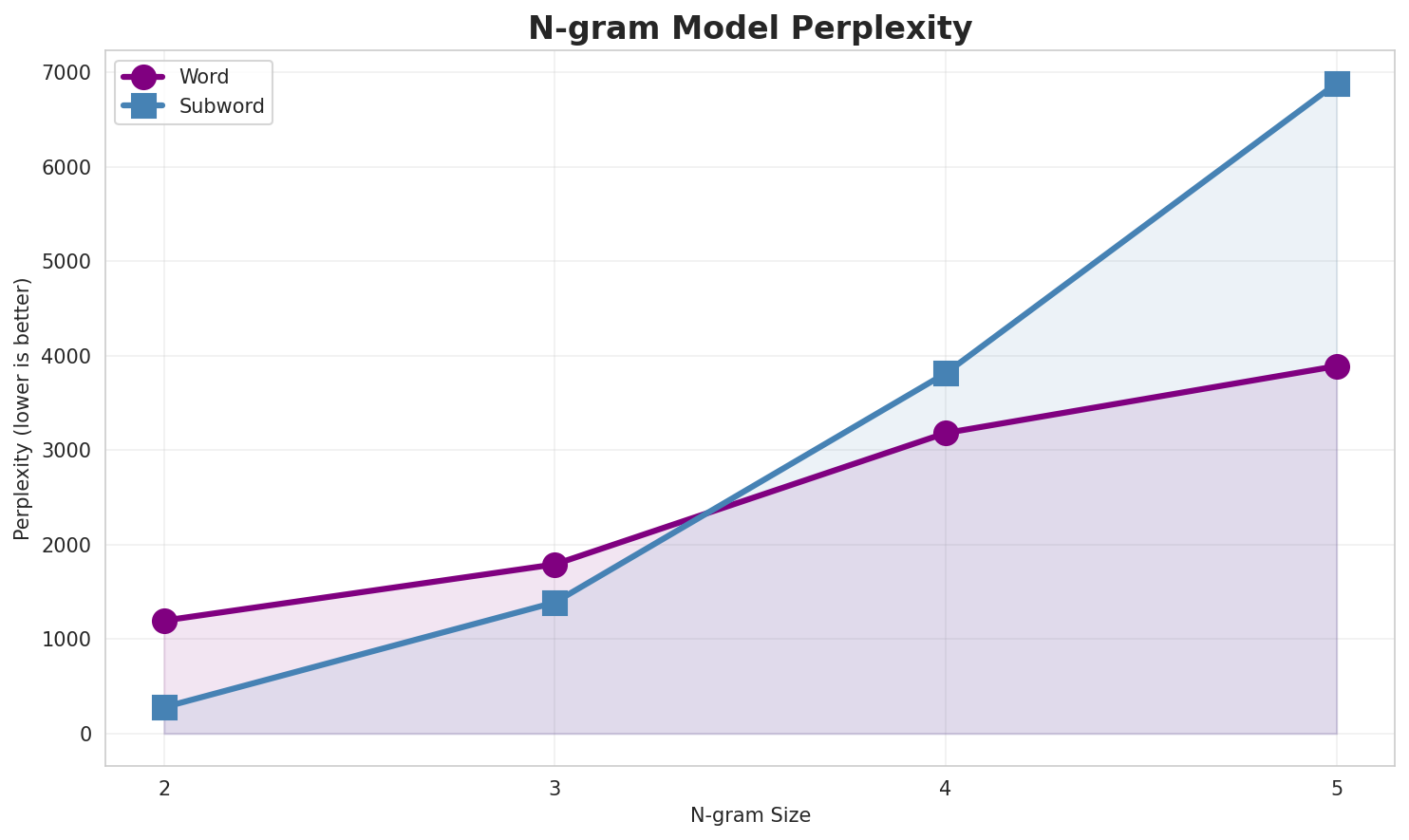
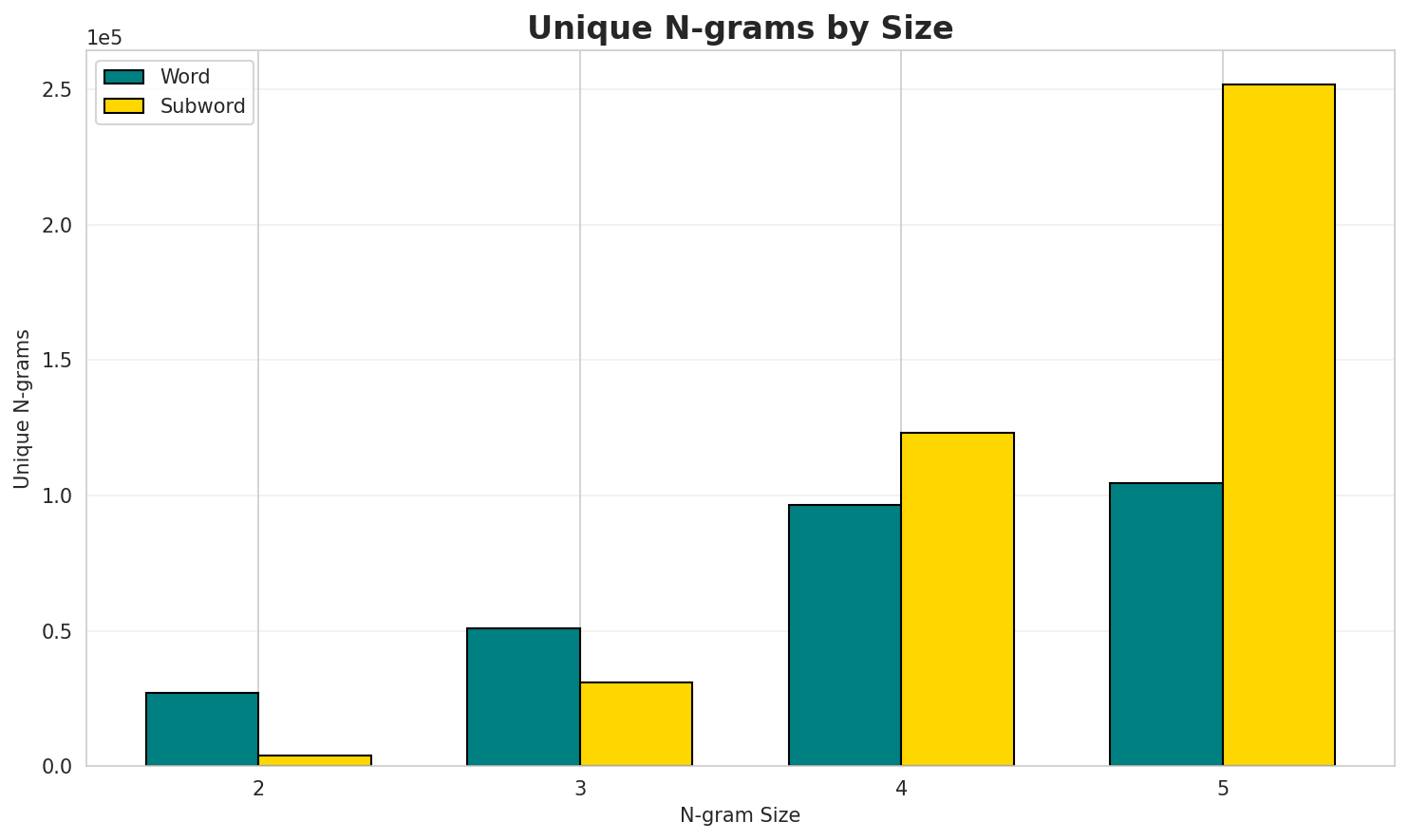
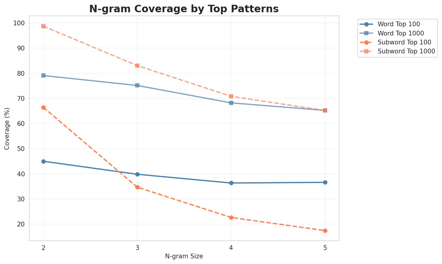
N-gram	Variant	Perplexity	Entropy	Unique N-grams	Top-100 Coverage	Top-1000 Coverage
2-gram	Word	1,196	10.22	27,047	45.0%	79.1%
2-gram	Subword	278 🏆	8.12	3,951	66.4%	98.7%
3-gram	Word	1,791	10.81	50,741	39.8%	75.1%
3-gram	Subword	1,389	10.44	30,764	34.7%	83.1%
4-gram	Word	3,181	11.64	96,325	36.3%	68.2%
4-gram	Subword	3,814	11.90	123,122	22.6%	70.8%
5-gram	Word	3,890	11.93	104,452	36.6%	65.2%
5-gram	Subword	6,884	12.75	251,758	17.4%	65.2%

Top 5 N-grams by Size

2-grams (Word):

Rank	N-gram	Count
1	ⵜⴳⵎⵉⴹⵉ ⵏ	30,065
2	ⵏ ⵓⵙⴳⴳⵯⴰⵙ	27,531
3	ⵓⵎⴹⴰⵏ ⵏ	26,944
4	ⵏ ⵉⵎⵣⴷⴰⵖⵏ	24,199
5	ⵜⵍⴽⵎ ⵜⴳⵎⵉⴹⵉ	24,115

3-grams (Word):

Rank	N-gram	Count
1	ⵜⵍⴽⵎ ⵜⴳⵎⵉⴹⵉ ⵏ	24,115
2	ⵓⵎⴹⴰⵏ ⵏ ⵉⵎⵣⴷⴰⵖⵏ	14,960
3	ⵜⴰⵎⴰⵜⵜⴰⵢⵜ ⵏ ⵓⵙⵖⵉⵡⵙ	14,959
4	ⵜⴰⵙⵎⵉⵔⵉⵜ ⵜⴰⵎⴰⵜⵜⴰⵢⵜ ⵏ	14,958
5	ⴳ ⵜⵍⴽⵎ ⵜⴳⵎⵉⴹⵉ	12,063

4-grams (Word):

Rank	N-gram	Count
1	ⵜⴰⵙⵎⵉⵔⵉⵜ ⵜⴰⵎⴰⵜⵜⴰⵢⵜ ⵏ ⵓⵙⵖⵉⵡⵙ	14,958
2	ⴳ ⵜⵍⴽⵎ ⵜⴳⵎⵉⴹⵉ ⵏ	12,063
3	ⵓⵎⴹⴰⵏ ⵏ ⵉⵎⵣⴷⴰⵖⵏ ⵏⵏⵙ	8,928
4	ⵉⵎⵣⴷⴰⵖⵏ ⵜⴰⵙⵎⵉⵔⵉⵜ ⵜⴰⵎⴰⵜⵜⴰⵢⵜ ⵏ	8,927
5	ⴰⵎⴰⵜⴰⵢ ⵏ ⵉⵎⵣⴷⴰⵖⵏ ⵜⴰⵙⵎⵉⵔⵉⵜ	8,927

5-grams (Word):

Rank	N-gram	Count
1	ⵏ ⵉⵎⵣⴷⴰⵖⵏ ⵜⴰⵙⵎⵉⵔⵉⵜ ⵜⴰⵎⴰⵜⵜⴰⵢⵜ ⵏ	8,927
2	ⴰⵎⴰⵜⴰⵢ ⵏ ⵉⵎⵣⴷⴰⵖⵏ ⵜⴰⵙⵎⵉⵔⵉⵜ ⵜⴰⵎⴰⵜⵜⴰⵢⵜ	8,927
3	ⵉⵎⵣⴷⴰⵖⵏ ⵜⴰⵙⵎⵉⵔⵉⵜ ⵜⴰⵎⴰⵜⵜⴰⵢⵜ ⵏ ⵓⵙⵖⵉⵡⵙ	8,927
4	ⵉⴹⴼⴰⵕ ⵓⵙⵓⵏ ⴰⴷ ⵉ ⵜⵔⴼⵉⵇⵜ	8,926
5	ⵍⵎⵖⵔⵉⴱ ⵉⴹⴼⴰⵕ ⵓⵙⵓⵏ ⴰⴷ ⵉ	8,926

2-grams (Subword):

Rank	N-gram	Count
1	ⵏ _	653,035
2	_ ⵏ	397,792
3	_ ⵜ	364,082
4	_ ⵉ	257,899
5	_ ⵓ	211,446

3-grams (Subword):

Rank	N-gram	Count
1	_ ⵏ _	291,650
2	_ ⵜ ⴰ	138,650
3	_ ⴳ _	115,983
4	ⵏ _ ⵉ	106,477
5	ⴰ ⵏ _	105,784

4-grams (Subword):

Rank	N-gram	Count
1	_ ⵏ _ ⵓ	86,083
2	ⵜ _ ⵏ _	65,334
3	_ ⵏ _ ⵉ	62,419
4	ⵏ _ ⵓ ⵙ	60,609
5	_ ⵏ _ ⵜ	57,983

5-grams (Subword):

Rank	N-gram	Count
1	_ ⵏ _ ⵓ ⵙ	51,067
2	ⵎ ⵣ ⴷ ⴰ ⵖ	45,993
3	ⴳ ⴳ ⵯ ⴰ ⵙ	36,185
4	ⵙ ⴳ ⴳ ⵯ ⴰ	36,178
5	_ ⵏ ⵏ ⴰ _	35,864

Key Findings

• Best Perplexity: 2-gram (subword) with 278
• Entropy Trend: Decreases with larger n-grams (more predictable)
• Coverage: Top-1000 patterns cover ~65% of corpus
• Recommendation: 4-gram or 5-gram for best predictive performance

---

3. Markov Chain Evaluation

Results

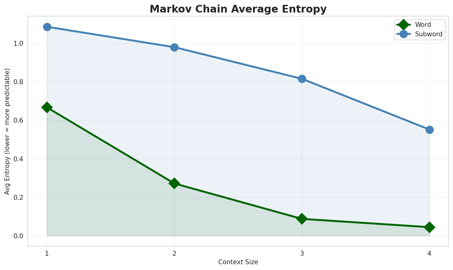
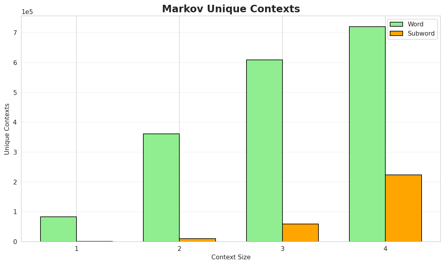
Context	Variant	Avg Entropy	Perplexity	Branching Factor	Unique Contexts	Predictability
1	Word	0.6673	1.588	4.36	83,258	33.3%
1	Subword	1.0864	2.123	8.88	1,091	0.0%
2	Word	0.2718	1.207	1.69	361,700	72.8%
2	Subword	0.9804	1.973	6.14	9,682	2.0%
3	Word	0.0879	1.063	1.19	608,815	91.2%
3	Subword	0.8161	1.761	3.76	59,433	18.4%
4	Word	0.0448 🏆	1.032	1.12	719,950	95.5%
4	Subword	0.5524	1.466	2.41	223,378	44.8%

Generated Text Samples (Word-based)

Below are text samples generated from each word-based Markov chain model:

Context Size 1:

1. ⵏ ⵜⴰⵚⵚⵓⵕⵜ ⵜⴰⵎⵏⴰⴹⵜ ⵏ 800 ⵏ ⵜⴰⵎⴹⵉⵜ ⵙ ⵜⴳⵎⵉⴹⵉ ⵏ ⵍⵎⵏⵣⵍ ⵜⴰⵙⴳⴰ ⵏ ⵓⵙⵍⵎⴷ 95 ⵏ
2. ⴳ ⵜⵍⴽⵎ ⵜⴳⵎⵉⴹⵉ ⵏ ⵜⵎⵍⵙⴰ ⵢⴰⴹⵏⵉ ⵣⵓⵏ ⴷ 11 ⵏ ⵢⵉⵡⵍ ⴰⵎⵣⵡⴰⵔⵓ 33 85 37 5
3. ⴷ ⵉⵔⴰⵔ ⵍⵎⵖⵔⵉⴱ ⵉⴹⴼⴰⵕ ⵓⵙⵓⵏ ⵉⵎⵓⵏⵏ ⵢⵉⵍⵉ ⴳ ⵓⵙⵉⴹⵏ ⴰⵎⴰⴷⴷⵓⴷ ⵏ ⵜⴳⵍⴷⵉⵜ ⵜⴰⵙⴰⵄⵓⴷⵉⵜ ⴳ ⵜⴳⵔⴰⵡⵜ ⵏ

Context Size 2:

1. ⵜⴳⵎⵉⴹⵉ ⵏ ⵎⴷⴷ ⵏⵏⴰ ⵥⴹⴰⵕⵏⵉⵏ ⵉ ⵜⵡⵓⵔⵉ 53 52 ⴳ ⴰⵢⵜ ⵄⵍⵍⴰ ⵏⵏⴰ ⴳ ⵍⵍⴰⵏ 5 ⵏ
2. ⵏ ⵓⵙⴳⴳⵯⴰⵙ démographiques et socio économiques de la population et de l habitat de ⵜⴰⵙⵎⵉⵔⵉⵜ ⵜⴰⵎⴰⵜⵜⴰⵢⵜ...
3. ⵓⵎⴹⴰⵏ ⵏ ⵉⵎⵣⴷⴰⵖⵏ ⵏⵏⵙ 75 ⵏ ⵜⵡⵜⵎⵉⵏ ⵜⴰⵡⵊⵉⵡⵉⵏ ⵉⵡⵍ ⴷ ⵜⴰⵔⵡⴰ ⴳ ⴳⴰⵏ ⵡⵉⵏⴰ ⵢⵉⵡⵍⵏ ⴳ ⵓⵙⵓⵏ

Context Size 3:

1. ⵜⵍⴽⵎ ⵜⴳⵎⵉⴹⵉ ⵏ ⵜⴰⵔⵙⴽⴽⵉⵍⵜ 50 98 ⴳⵔ ⵉⵔⴱⴰⵏ ⴷ ⵜⵔⴱⴰⵜⵉⵏ ⵏⵏⴰ ⵖⵓⵔ ⴳⵔ 6 ⴷ 11 ⵏ ⵓⵙⴳⴳⵯⴰⵙ
2. ⵓⵎⴹⴰⵏ ⵏ ⵉⵎⵣⴷⴰⵖⵏ ⵏⵏⵙ 122 ⵏ ⵓⵎⵣⴷⴰⵖ ⴳ ⵓⵙⵉⴹⵏ ⴰⵎⴰⴷⴷⵓⴷ ⵏ ⵓⵙⴳⴳⵯⴰⵙ démographiques et socio économiques de la
3. ⵜⴰⵎⴰⵜⵜⴰⵢⵜ ⵏ ⵓⵙⵖⵉⵡⵙ ⴰⵕⵛⵉⴼ 14 ⵖⵓⵛⵜ ⵜⵉⵙⵏⴰⴷⴷⴰⴷⵉⵏ ⵜⵉⵙⵏⴰⴷⴷⴰⴷⵉⵏ ⵜⵉⵎⴰⵜⴰⵢⵉⵏ ⵉⴳⴳⵯⵉⵣ ⵓⵎⴹⴰⵏ ⵏ ⵉⵎⵣⴷⴰⵖⵏ ⵏ ⵜⴰⵖⵣⵓⵜ ⵙ...

Context Size 4:

1. ⵜⴰⵙⵎⵉⵔⵉⵜ ⵜⴰⵎⴰⵜⵜⴰⵢⵜ ⵏ ⵓⵙⵖⵉⵡⵙ ⴰⵕⵛⵉⴼ 14 ⵖⵓⵛⵜ ⵜⵉⵙⵏⴰⴷⴷⴰⴷⵉⵏ ⵜⵉⵙⵏⴰⴷⴷⴰⴷⵉⵏ ⵜⵉⵎⴰⵜⴰⵢⵉⵏ ⵉⴳⴳⵯⵉⵣ ⵓⵎⴹⴰⵏ ⵏ ⵉⵎⵣⴷⴰⵖⵏ ⵏ...
2. ⴳ ⵜⵍⴽⵎ ⵜⴳⵎⵉⴹⵉ ⵏ ⵎⴷⴷ ⵏⵏⴰ ⵥⴹⴰⵕⵏⵉⵏ ⵉ ⵜⵡⵓⵔⵉ 55 29 ⴳ ⴰⵢⵜ ⴱⵏ ⵄⴱⴱⵓ ⴰⵔ ⵏⵉⵜ ⵙⵡⵓⵔⵉⵏ ⵏⵉⵖ
3. ⵓⵎⴹⴰⵏ ⵏ ⵉⵎⵣⴷⴰⵖⵏ ⵏⵏⵙ 390 ⵏ ⵓⵎⵣⴷⴰⵖ ⴳ ⵓⵙⵉⴹⵏ ⴰⵎⴰⴷⴷⵓⴷ ⵏ ⵓⵙⴳⴳⵯⴰⵙ démographiques et socio économiques de la...

Generated Text Samples (Subword-based)

Below are text samples generated from each subword-based Markov chain model:

Context Size 1:

1. _ⵜⴰⵢⵢⵉⵏⴰⵔ_ⴱⵜⴰⵏ_ⵓ
2. ⴰⵖⵉⵜ_ⵖⵜ_ⵇⵏ_ⴳ_non
3. ⵏ_ⵉⵇⵜⴰ_ⵏ_ⵓⵎⴹⵏ_ⴼⵜ

Context Size 2:

1. ⵏ_ⴷ_ⵉⴳⴳⵉⵙⵙ_3_ⴰⵍ_ⴰ
2. _ⵏ_ⴰⵎⴰⵏ_ⴳ_ⵓⵙⵙⴰⵖⵏ_
3. _ⵜⵡⵓⵔ_6_ⴽⵓⴷⴰⵖ,_ⵉⵥ

Context Size 3:

1. _ⵏ_ⵜⴰⵙⵡⵉⵏ_ⵉⵙⴽⴰⵔⵏⵜ_
2. _ⵜⴰⵡⵓⵔⵉ_4.52%_ⴳⵔ_6
3. _ⴳ_ⵍⵍⴰⵏ_ⵡⵉⵏ:_ⵉⵡⵜⵎⵉ

Context Size 4:

1. _ⵏ_ⵓⵍⴰ_ⴳ_ⴳⴰⵏ_ⵡⵉⵏⴰ_ⵢ
2. ⵜ_ⵏ_ⵓⵙⵖⵉⵡⵙ._ⴰⵕⵛⵉⴼ,_
3. _ⵏ_ⵉⵡⵜⵎⴰⵏ_ⴷ_24.85,_

Key Findings

• Best Predictability: Context-4 (word) with 95.5% predictability
• Branching Factor: Decreases with context size (more deterministic)
• Memory Trade-off: Larger contexts require more storage (223,378 contexts)
• Recommendation: Context-3 or Context-4 for text generation

---

4. Vocabulary Analysis

Statistics

Metric	Value
Vocabulary Size	35,191
Total Tokens	2,431,531
Mean Frequency	69.10
Median Frequency	4
Frequency Std Dev	1880.39

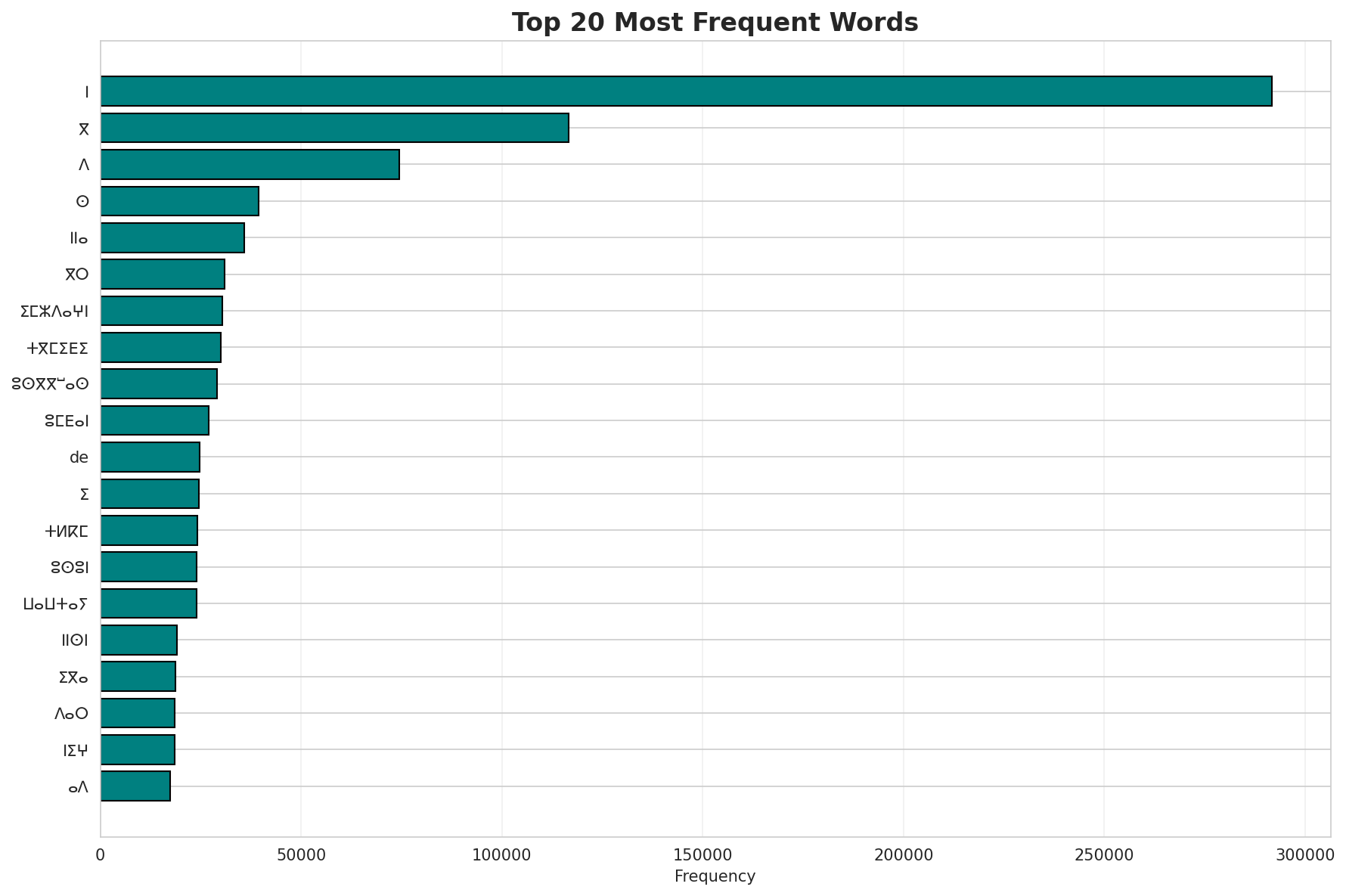
Most Common Words

Rank	Word	Frequency
1	ⵏ	291,759
2	ⴳ	116,564
3	ⴷ	74,542
4	ⵙ	39,445
5	ⵏⵏⴰ	35,886
6	ⴳⵔ	30,891
7	ⵉⵎⵣⴷⴰⵖⵏ	30,462
8	ⵜⴳⵎⵉⴹⵉ	30,068
9	ⵓⵙⴳⴳⵯⴰⵙ	29,018
10	ⵓⵎⴹⴰⵏ	27,041

Least Common Words (from vocabulary)

Rank	Word	Frequency
1	ⵓⵎⵙⵙⵉⵥⵉⵕ	2
2	ⵜⵙⵔⴽⵎⵉⵏ	2
3	ⵓⵎⵢⴰⴱⴰ	2
4	fourth	2
5	ⵜⴰⴱⵔⵓⵙⵉⵜ	2
6	ⵜⴰⵙⵏⴽⵜⴰ	2
7	ⵜⵉⵣⵎⵣⴰⵏⵉⵏ	2
8	ⵜⴰⴷⵓⵥⴽⵉⵡⵜ	2
9	ⴰⵎⵥⵕⴷⴳⴰⵔ	2
10	ⵜⴰⵥⵕⵎⴰⵔⴽⵙⵉⵜ	2

Zipf's Law Analysis

Metric	Value
Zipf Coefficient	1.2553
R² (Goodness of Fit)	0.991414
Adherence Quality	excellent

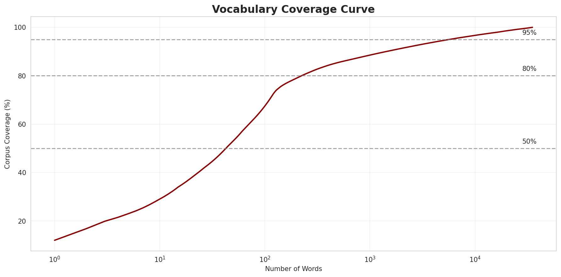
Coverage Analysis

Top N Words	Coverage
Top 100	67.5%
Top 1,000	88.5%
Top 5,000	94.6%
Top 10,000	96.7%

Key Findings

• Zipf Compliance: R²=0.9914 indicates excellent adherence to Zipf's law
• High Frequency Dominance: Top 100 words cover 67.5% of corpus
• Long Tail: 25,191 words needed for remaining 3.3% coverage

---

5. Word Embeddings Evaluation

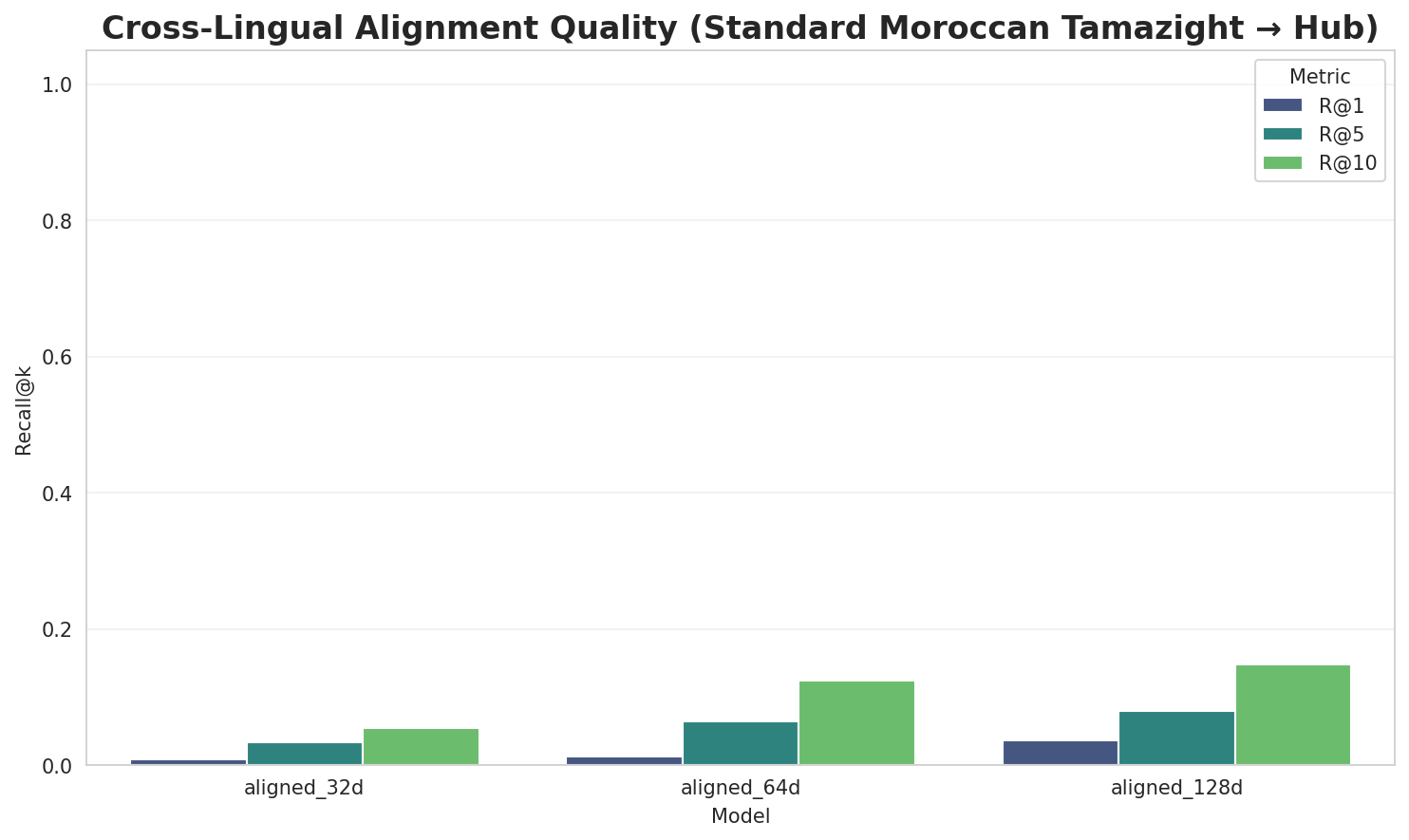
5.1 Cross-Lingual Alignment

5.2 Model Comparison

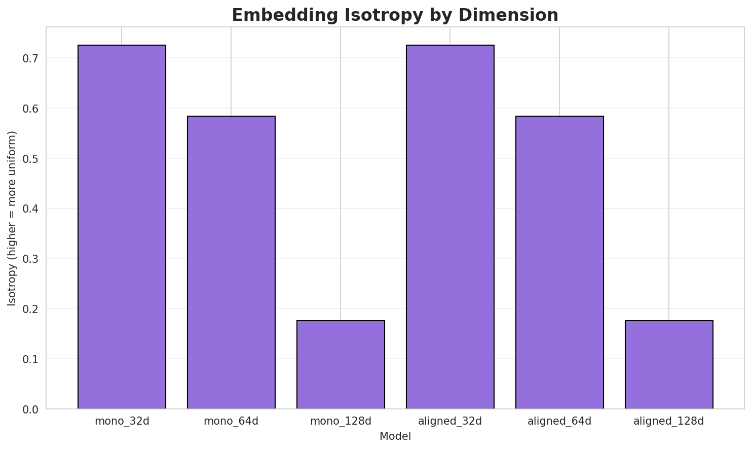
Model	Dimension	Isotropy	Semantic Density	Alignment R@1	Alignment R@10
mono_32d	32	0.7259 🏆	0.3600	N/A	N/A
mono_64d	64	0.5835	0.3114	N/A	N/A
mono_128d	128	0.1766	0.3125	N/A	N/A
aligned_32d	32	0.7259	0.3745	0.0080	0.0540
aligned_64d	64	0.5835	0.3265	0.0120	0.1240
aligned_128d	128	0.1766	0.3192	0.0360	0.1480

Key Findings

• Best Isotropy: mono_32d with 0.7259 (more uniform distribution)
• Semantic Density: Average pairwise similarity of 0.3340. Lower values indicate better semantic separation.
• Alignment Quality: Aligned models achieve up to 3.6% R@1 in cross-lingual retrieval.
• Recommendation: 128d aligned for best cross-lingual performance

---

6. Morphological Analysis (Experimental)

This section presents an automated morphological analysis derived from the statistical divergence between word-level and subword-level models. By analyzing where subword predictability spikes and where word-level coverage fails, we can infer linguistic structures without supervised data.

6.1 Productivity & Complexity

Metric	Value	Interpretation	Recommendation
Productivity Index	5.000	High morphological productivity	Reliable analysis
Idiomaticity Gap	0.001	Low formulaic content	-

6.2 Affix Inventory (Productive Units)

These are the most productive prefixes and suffixes identified by sampling the vocabulary for global substitutability patterns. A unit is considered an affix if stripping it leaves a valid stem that appears in other contexts.

Productive Prefixes

Prefix	Examples
-ⵜ	ⵜⵉⵎⵙⵙⵉ, ⵜⴳⵎⴰⵎⵜ, ⵜⵛⴰⵡⵉⵜ
-ⵜⴰ	ⵜⴰⵎⴰⴽⵓⴷⵜ, ⵜⴰⴱⵕⵕⴰⵏⵉⵢⵜ, ⵜⴰⵇⵇⴰⵢⵜ
-ⵉ	ⵉⵙⵙⵏⵄⴰⵜ, ⵉⴳⵯⵔⵔⴰⵎⵏ, ⵉⵊ
-ⴰ	ⴰⵎⵙⵏⴽⴰⵔ, ⴰⵜⵉⵍⵉⴼⵉⵣⵢⵓⵏ, ⴰⵎⵖⵔⵉⴱⵉⵢ
-ⵓ	ⵓⵊⵔⵉ, ⵓⴳⵜⴷⵉⵙ, ⵓⵔⵔⴰⵡ
-ⵜⵉ	ⵜⵉⵎⵙⵙⵉ, ⵜⵉⵎⵥⴰⵕⵕⵓⵕⵉⵏ, ⵜⵉⵎⵥⵍⴰⵢⵉⵏ
-ⵍ	ⵍⵃⵓⵎⴰ, ⵍⵡⴰⴷ, ⵍⴳⵯⵍⵍⴰ
-ⵉⵎ	ⵉⵎⵥⵉⵏⵛⵓⵜⴰⵏⴱⵉⵔ, ⵉⵎⵢⴰⴳⴰⵔ, ⵉⵎⴷⴰⵏ

Productive Suffixes

Suffix	Examples
-ⵏ	ⴽⵔⵓⵛⵏ, ⵉⴳⵯⵔⵔⴰⵎⵏ, ⵜⵉⵎⵥⴰⵕⵕⵓⵕⵉⵏ
-ⵜ	ⵜⴳⵎⴰⵎⵜ, ⵜⵛⴰⵡⵉⵜ, ⵉⵙⵙⵏⵄⴰⵜ
-ⵉⵏ	ⵜⵉⵎⵥⴰⵕⵕⵓⵕⵉⵏ, ⵣⵣⵏⵣⴰⵏⵉⵏ, ⵜⵉⵎⵥⵍⴰⵢⵉⵏ
-ⴰ	ⴱⵓⴷⴰ, ⵊⴰⵎⴰⵢⴽⴰ, ⵍⵃⵓⵎⴰ
-ⵉ	ⵜⵉⵎⵙⵙⵉ, ⵓⵊⵔⵉ, ⵏⵜⵜⵉⵏⵉ
-ⴰⵏ	ⵉⴱⵇⵇⴰⵏ, ⵎⵛⴰⵛⴽⴰⵏ, ⵉⵎⴷⴰⵏ
-ⵉⵜ	ⵜⵛⴰⵡⵉⵜ, ⵜⴰⴷⵉⵏⴰⵎⵉⵜ, ⴱⵓⵜⵓⵏⴼⵉⵜ
-ⵔ	ⴰⵎⵙⵏⴽⴰⵔ, ⵜⵜⵔ, ⵉⵎⵥⵉⵏⵛⵓⵜⴰⵏⴱⵉⵔ

6.3 Bound Stems (Lexical Roots)

Bound stems are high-frequency subword units that are semantically cohesive but rarely appear as standalone words. These often correspond to the 'core' of a word that requires inflection or derivation to be valid.

Stem	Cohesion	Substitutability	Examples
ⴰⴷⴷⴰ	1.60x	54 contexts	ⵜⴰⴷⴷⴰ, ⴰⴷⴷⴰⴳ, ⵢⴰⴷⴷⴰ
ⵡⵓⵔⵉ	1.73x	38 contexts	ⵜⵡⵓⵔⵉ, ⵜⵙⵡⵓⵔⵉ, ⴰⵙⵡⵓⵔⵉ
ⴳⴳⴰⵔ	1.70x	24 contexts	ⵉⴳⴳⴰⵔ, ⴳⴳⴰⵔⵏ, ⵓⴳⴳⴰⵔ
ⵓⴳⴳⴰ	1.65x	24 contexts	ⵢⵓⴳⴳⴰ, ⵜⵓⴳⴳⴰ, ⵓⴳⴳⴰⵏ
ⵜⵜⴰⵢ	1.71x	19 contexts	ⴰⵜⵜⴰⵢ, ⵓⵡⵜⵜⴰⵢ, ⵓⵏⵜⵜⴰⵢ
ⴰⵜⵜⴰ	1.62x	22 contexts	ⴰⵜⵜⴰⵢ, ⵎⴰⵜⵜⴰ, ⴰⵜⵜⴰⵖ
ⵎⵉⵔⵉ	1.54x	21 contexts	ⵉⵎⵉⵔⵉ, ⵓⵎⵉⵔⵉⴳ, ⵜⵎⵉⵔⵉⵜ
ⴷⴷⴰⴷ	1.66x	16 contexts	ⵃⴷⴷⴰⴷ, ⵓⴷⴷⴰⴷ, ⵉⴷⴷⴰⴷ
ⴰⵎⴰⵜ	1.50x	17 contexts	ⴰⵎⴰⵜⵓ, ⴰⵎⴰⵜⴰ, ⴰⵎⴰⵜⵜⵓ
ⵙⵍⵎⴷ	1.69x	12 contexts	ⴰⵙⵍⵎⴷ, ⵓⵙⵍⵎⴷ, ⵙⵍⵎⴷⵏ
ⵉⵔⵉⵜ	1.59x	14 contexts	ⵜⵉⵔⵉⵜ, ⵙⵉⵔⵉⵜ, ⵙⴱⵉⵔⵉⵜ
ⴰⵢⵉⵏ	1.86x	9 contexts	ⴼⵍⴰⵢⵉⵏ, ⵜⵎⴷⴰⵢⵉⵏ, ⵜⵓⵎⴰⵢⵉⵏ

6.4 Affix Compatibility (Co-occurrence)

This table shows which prefixes and suffixes most frequently co-occur on the same stems, revealing the 'stacking' rules of the language's morphology.

Prefix	Suffix	Frequency	Examples
-ⵜ	-ⵜ	684 words	ⵜⴰⴱⵔⵓⵜⵉⵙⵜⴰⵏⵜⵉⵜ, ⵜⴰⵏⵓⵍⴼⵓⵜ
-ⵉ	-ⵏ	523 words	ⵉⴼⵓⵄⵣⵏ, ⵉⵎⵙⴷⵎⴰⵔⵏ
-ⵜ	-ⵏ	379 words	ⵜⵢⴰⴼⵓⵜⵉⵏ, ⵜⵉⵕⵚⵍⵉⵢⵉⵏ
-ⵜ	-ⵉⵏ	331 words	ⵜⵢⴰⴼⵓⵜⵉⵏ, ⵜⵉⵕⵚⵍⵉⵢⵉⵏ
-ⵜ	-ⵉⵜ	130 words	ⵜⴰⴱⵔⵓⵜⵉⵙⵜⴰⵏⵜⵉⵜ, ⵜⴰⵊⵓⴳⵕⴰⴼⵉⵜ
-ⵍ	-ⴰ	101 words	ⵍⴼⴰⵢⴹⴰ, ⵍⴱⵕⵕⴰⵏⵢⵢⴰ
-ⵜ	-ⴰ	74 words	ⵜⵜⵓⴱⵏⴰ, ⵜⴰⵎⴰ
-ⵉ	-ⴰⵏ	63 words	ⵉⵎⵛⴰⵛⴽⴰⵏ, ⵉⵡⴷⴰⵏ
-ⴰ	-ⵏ	58 words	ⴰⵀⵉⵍⵏ, ⴰⵎⴽⴰⵏ
-ⴰ	-ⵉ	47 words	ⴰⵎⵣⴳⵉ, ⴰⴷⵡⴰⵍⵉ

6.5 Recursive Morpheme Segmentation

Using Recursive Hierarchical Substitutability, we decompose complex words into their constituent morphemes. This approach handles nested affixes (e.g., prefix-prefix-root-suffix).

Word	Suggested Split	Confidence	Stem
ⵜⵉⵔⵍⵓⴳⵏⴰⵏⵉⵏ	ⵜⵉⵔⵍⵓⴳⵏⴰ-ⵏ-ⵉⵏ	7.5	ⵏ
ⵜⴳⵔⴰⵖⵍⴰⵏⵉⵏ	ⵜⴳⵔⴰⵖⵍⴰ-ⵏ-ⵉⵏ	7.5	ⵏ
ⵜⵜⵄⵕⵕⴱⵏⵉⵏ	ⵜⵜⵄⵕⵕⴱ-ⵏ-ⵉⵏ	7.5	ⵏ
ⵉⵜⵜⴰⵡⵙⵙⴰⵏⵏ	ⵉⵜⵜⴰⵡⵙⵙⴰ-ⵏ-ⵏ	7.5	ⵏ
ⵉⵎⵖⵔⴰⴷⴰⵏⵏ	ⵉⵎⵖⵔⴰⴷⴰ-ⵏ-ⵏ	7.5	ⵏ
ⵜⵉⵎⴰⵙⵉⵏⵉⵏ	ⵜⵉⵎⴰⵙ-ⵉⵏ-ⵉⵏ	7.5	ⵉⵏ
ⵉⵙⵉⵏⴰⵔⵢⵓⵜⵏ	ⵉⵙⵉⵏⴰⵔⵢⵓ-ⵜ-ⵏ	7.5	ⵜ
ⵜⵉⵙⵏⵛⵏⵢⴰⵍⴰⵏⵉⵏ	ⵜⵉⵙⵏⵛⵏⵢⴰⵍ-ⴰⵏ-ⵉⵏ	7.5	ⴰⵏ
ⴽⵔⵉⵙⵜⵢⴰⵏⵓ	ⴽⵔⵉⵙⵜⵢⴰ-ⵏ-ⵓ	7.5	ⵏ
ⵜⵜⵓⵙⵎⵔⴰⵙⵏⵉⵏ	ⵜⵜⵓⵙⵎⵔⴰⵙ-ⵏ-ⵉⵏ	7.5	ⵏ
ⵜⵉⵎⵢⴰⵇⴰⵏⵉⵏ	ⵜⵉⵎⵢⴰⵇ-ⴰⵏ-ⵉⵏ	7.5	ⴰⵏ
ⵜⵉⵏⵎⴹⴰⵏⵉⵏ	ⵜⵉⵏⵎⴹ-ⴰⵏ-ⵉⵏ	7.5	ⴰⵏ
ⵜⵜⵡⴰⵙⵙⴰⵏⵏⵜ	ⵜⵜⵡⴰⵙⵙⴰⵏ-ⵏ-ⵜ	7.5	ⵏ
ⵉⵙⵜⵓⴷⵢⵓⵜⵏ	ⵉⵙⵜⵓⴷⵢⵓ-ⵜ-ⵏ	7.5	ⵜ
ⵉⵜⵜⵓⵙⵖⵥⵏⵏ	ⵉⵜⵜⵓⵙⵖⵥ-ⵏ-ⵏ	7.5	ⵏ

6.6 Linguistic Interpretation

Automated Insight: The language Standard Moroccan Tamazight shows high morphological productivity. The subword models are significantly more efficient than word models, suggesting a rich system of affixation or compounding.

---

7. Summary & Recommendations

Production Recommendations

Component	Recommended	Rationale
Tokenizer	64k BPE	Best compression (3.84x)
N-gram	2-gram	Lowest perplexity (278)
Markov	Context-4	Highest predictability (95.5%)
Embeddings	100d	Balanced semantic capture and isotropy

---

Appendix: Metrics Glossary & Interpretation Guide

This section provides definitions, intuitions, and guidance for interpreting the metrics used throughout this report.

Tokenizer Metrics

Compression Ratio

Definition: The ratio of characters to tokens (chars/token). Measures how efficiently the tokenizer represents text.

Intuition: Higher compression means fewer tokens needed to represent the same text, reducing sequence lengths for downstream models. A 3x compression means ~3 characters per token on average.

What to seek: Higher is generally better for efficiency, but extremely high compression may indicate overly aggressive merging that loses morphological information.

Average Token Length (Fertility)

Definition: Mean number of characters per token produced by the tokenizer.

Intuition: Reflects the granularity of tokenization. Longer tokens capture more context but may struggle with rare words; shorter tokens are more flexible but increase sequence length.

What to seek: Balance between 2-5 characters for most languages. Arabic/morphologically-rich languages may benefit from slightly longer tokens.

Unknown Token Rate (OOV Rate)

Definition: Percentage of tokens that map to the unknown/UNK token, indicating words the tokenizer cannot represent.

Intuition: Lower OOV means better vocabulary coverage. High OOV indicates the tokenizer encounters many unseen character sequences.

What to seek: Below 1% is excellent; below 5% is acceptable. BPE tokenizers typically achieve very low OOV due to subword fallback.

N-gram Model Metrics

Perplexity

Definition: Measures how "surprised" the model is by test data. Mathematically: 2^(cross-entropy). Lower values indicate better prediction.

Intuition: If perplexity is 100, the model is as uncertain as if choosing uniformly among 100 options at each step. A perplexity of 10 means effectively choosing among 10 equally likely options.

What to seek: Lower is better. Perplexity decreases with larger n-grams (more context). Values vary widely by language and corpus size.

Entropy

Definition: Average information content (in bits) needed to encode the next token given the context. Related to perplexity: perplexity = 2^entropy.

Intuition: High entropy means high uncertainty/randomness; low entropy means predictable patterns. Natural language typically has entropy between 1-4 bits per character.

What to seek: Lower entropy indicates more predictable text patterns. Entropy should decrease as n-gram size increases.

Coverage (Top-K)

Definition: Percentage of corpus occurrences explained by the top K most frequent n-grams.

Intuition: High coverage with few patterns indicates repetitive/formulaic text; low coverage suggests diverse vocabulary usage.

What to seek: Depends on use case. For language modeling, moderate coverage (40-60% with top-1000) is typical for natural text.

Markov Chain Metrics

Average Entropy

Definition: Mean entropy across all contexts, measuring average uncertainty in next-word prediction.

Intuition: Lower entropy means the model is more confident about what comes next. Context-1 has high entropy (many possible next words); Context-4 has low entropy (few likely continuations).

What to seek: Decreasing entropy with larger context sizes. Very low entropy (<0.1) indicates highly deterministic transitions.

Branching Factor

Definition: Average number of unique next tokens observed for each context.

Intuition: High branching = many possible continuations (flexible but uncertain); low branching = few options (predictable but potentially repetitive).

What to seek: Branching factor should decrease with context size. Values near 1.0 indicate nearly deterministic chains.

Predictability

Definition: Derived metric: (1 - normalized_entropy) × 100%. Indicates how deterministic the model's predictions are.

Intuition: 100% predictability means the next word is always certain; 0% means completely random. Real text falls between these extremes.

What to seek: Higher predictability for text generation quality, but too high (>98%) may produce repetitive output.

Vocabulary & Zipf's Law Metrics

Zipf's Coefficient

Definition: The slope of the log-log plot of word frequency vs. rank. Zipf's law predicts this should be approximately -1.

Intuition: A coefficient near -1 indicates the corpus follows natural language patterns where a few words are very common and most words are rare.

What to seek: Values between -0.8 and -1.2 indicate healthy natural language distribution. Deviations may suggest domain-specific or artificial text.

R² (Coefficient of Determination)

Definition: Measures how well the linear fit explains the frequency-rank relationship. Ranges from 0 to 1.

Intuition: R² near 1.0 means the data closely follows Zipf's law; lower values indicate deviation from expected word frequency patterns.

What to seek: R² > 0.95 is excellent; > 0.99 indicates near-perfect Zipf adherence typical of large natural corpora.

Vocabulary Coverage

Definition: Cumulative percentage of corpus tokens accounted for by the top N words.

Intuition: Shows how concentrated word usage is. If top-100 words cover 50% of text, the corpus relies heavily on common words.

What to seek: Top-100 covering 30-50% is typical. Higher coverage indicates more repetitive text; lower suggests richer vocabulary.

Word Embedding Metrics

Isotropy

Definition: Measures how uniformly distributed vectors are in the embedding space. Computed as the ratio of minimum to maximum singular values.

Intuition: High isotropy (near 1.0) means vectors spread evenly in all directions; low isotropy means vectors cluster in certain directions, reducing expressiveness.

What to seek: Higher isotropy generally indicates better-quality embeddings. Values > 0.1 are reasonable; > 0.3 is good. Lower-dimensional embeddings tend to have higher isotropy.

Average Norm

Definition: Mean magnitude (L2 norm) of word vectors in the embedding space.

Intuition: Indicates the typical "length" of vectors. Consistent norms suggest stable training; high variance may indicate some words are undertrained.

What to seek: Relatively consistent norms across models. The absolute value matters less than consistency (low std deviation).

Cosine Similarity

Definition: Measures angular similarity between vectors, ranging from -1 (opposite) to 1 (identical direction).

Intuition: Words with similar meanings should have high cosine similarity. This is the standard metric for semantic relatedness in embeddings.

What to seek: Semantically related words should score > 0.5; unrelated words should be near 0. Synonyms often score > 0.7.

t-SNE Visualization

Definition: t-Distributed Stochastic Neighbor Embedding - a dimensionality reduction technique that preserves local structure for visualization.

Intuition: Clusters in t-SNE plots indicate groups of semantically related words. Spread indicates vocabulary diversity; tight clusters suggest semantic coherence.

What to seek: Meaningful clusters (e.g., numbers together, verbs together). Avoid over-interpreting distances - t-SNE preserves local, not global, structure.

General Interpretation Guidelines

1. Compare within model families: Metrics are most meaningful when comparing models of the same type (e.g., 8k vs 64k tokenizer).
2. Consider trade-offs: Better performance on one metric often comes at the cost of another (e.g., compression vs. OOV rate).
3. Context matters: Optimal values depend on downstream tasks. Text generation may prioritize different metrics than classification.
4. Corpus influence: All metrics are influenced by corpus characteristics. Wikipedia text differs from social media or literature.
5. Language-specific patterns: Morphologically rich languages (like Arabic) may show different optimal ranges than analytic languages.

Visualizations Index

Visualization	Description
Tokenizer Compression	Compression ratios by vocabulary size
Tokenizer Fertility	Average token length by vocabulary
Tokenizer OOV	Unknown token rates
Tokenizer Total Tokens	Total tokens by vocabulary
N-gram Perplexity	Perplexity by n-gram size
N-gram Entropy	Entropy by n-gram size
N-gram Coverage	Top pattern coverage
N-gram Unique	Unique n-gram counts
Markov Entropy	Entropy by context size
Markov Branching	Branching factor by context
Markov Contexts	Unique context counts
Zipf's Law	Frequency-rank distribution with fit
Vocab Frequency	Word frequency distribution
Top 20 Words	Most frequent words
Vocab Coverage	Cumulative coverage curve
Embedding Isotropy	Vector space uniformity
Embedding Norms	Vector magnitude distribution
Embedding Similarity	Word similarity heatmap
Nearest Neighbors	Similar words for key terms
t-SNE Words	2D word embedding visualization
t-SNE Sentences	2D sentence embedding visualization
Position Encoding	Encoding method comparison
Model Sizes	Storage requirements
Performance Dashboard	Comprehensive performance overview

---

About This Project

Data Source

Models trained on wikipedia-monthly - a monthly snapshot of Wikipedia articles across 300+ languages.

Project

A project by Wikilangs - Open-source NLP models for every Wikipedia language.

Maintainer

Omar Kamali - Omneity Labs

Citation

If you use these models in your research, please cite:

@misc{wikilangs2025,
  author = {Kamali, Omar},
  title = {Wikilangs: Open NLP Models for Wikipedia Languages},
  year = {2025},
  doi = {10.5281/zenodo.18073153},
  publisher = {Zenodo},
  url = {https://huggingface.co/wikilangs}
  institution = {Omneity Labs}
}

License

MIT License - Free for academic and commercial use.

Links

• 🌐 Website: wikilangs.org
• 🤗 Models: huggingface.co/wikilangs
• 📊 Data: wikipedia-monthly
• 👤 Author: Omar Kamali
• 🤝 Sponsor: Featherless AI

---

Generated by Wikilangs Models Pipeline

Report Date: 2026-01-11 05:56:32