README.md

metadata

language: fj
language_name: Fijian
language_family: austronesian_oceanic_other
tags:
  - wikilangs
  - nlp
  - tokenizer
  - embeddings
  - n-gram
  - markov
  - wikipedia
  - feature-extraction
  - sentence-similarity
  - tokenization
  - n-grams
  - markov-chain
  - text-mining
  - fasttext
  - babelvec
  - vocabulous
  - vocabulary
  - monolingual
  - family-austronesian_oceanic_other
license: mit
library_name: wikilangs
pipeline_tag: text-generation
datasets:
  - omarkamali/wikipedia-monthly
dataset_info:
  name: wikipedia-monthly
  description: Monthly snapshots of Wikipedia articles across 300+ languages
metrics:
  - name: best_compression_ratio
    type: compression
    value: 4.558
  - name: best_isotropy
    type: isotropy
    value: 0.3441
  - name: vocabulary_size
    type: vocab
    value: 0
generated: 2026-01-04T00:00:00.000Z

Fijian - Wikilangs Models

Comprehensive Research Report & Full Ablation Study

This repository contains NLP models trained and evaluated by Wikilangs, specifically on Fijian Wikipedia data. We analyze tokenizers, n-gram models, Markov chains, vocabulary statistics, and word embeddings.

📋 Repository Contents

Models & Assets

• Tokenizers (8k, 16k, 32k, 64k)
• N-gram models (2, 3, 4, 5-gram)
• Markov chains (context of 1, 2, 3, 4 and 5)
• Subword N-gram and Markov chains
• Embeddings in various sizes and dimensions (aligned and unaligned)
• Language Vocabulary
• Language Statistics

Analysis and Evaluation

• 1. Tokenizer Evaluation
• 2. N-gram Model Evaluation
• 3. Markov Chain Evaluation
• 4. Vocabulary Analysis
• 5. Word Embeddings Evaluation
• 6. Morphological Analysis (Experimental)
• 7. Summary & Recommendations
• Metrics Glossary
• Visualizations Index

---

1. Tokenizer Evaluation

Results

Vocab Size	Compression	Avg Token Len	UNK Rate	Total Tokens
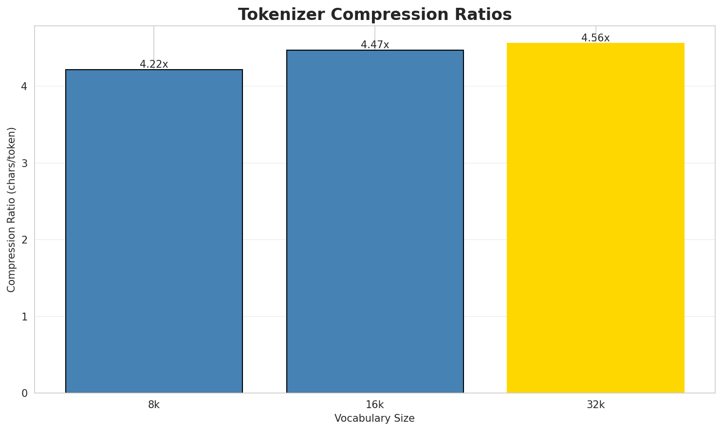
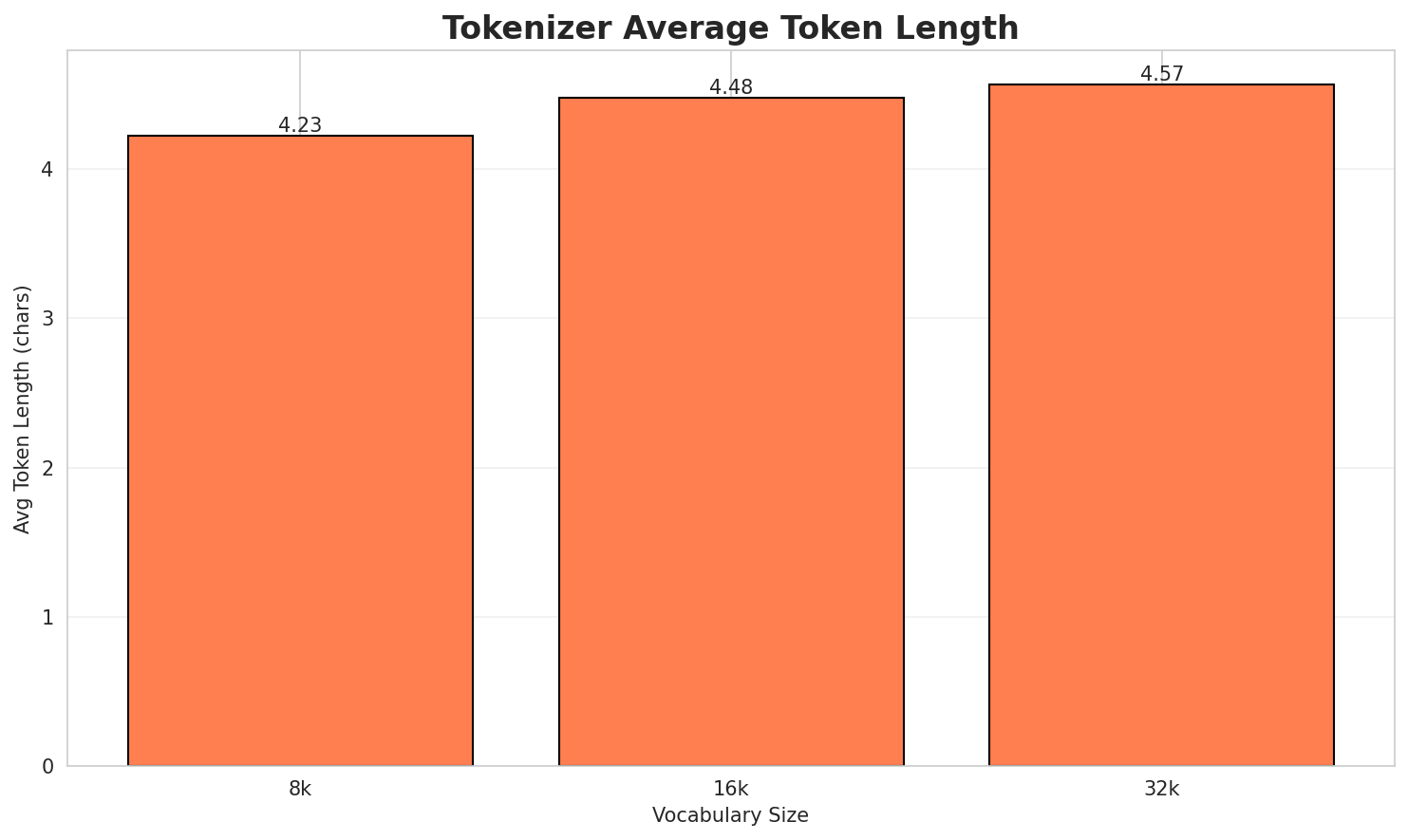
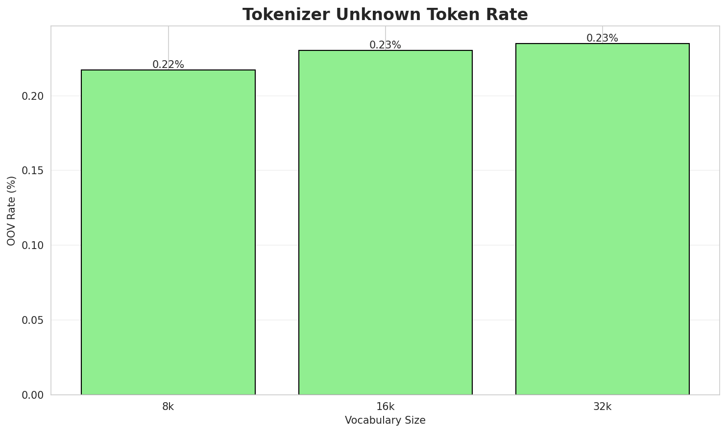
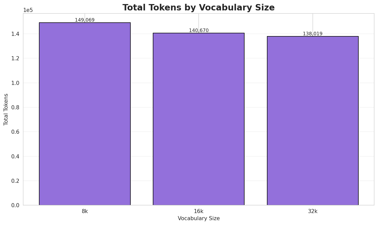
8k	4.221x	4.23	0.2173%	149,069
16k	4.473x	4.48	0.2303%	140,670
32k	4.558x 🏆	4.57	0.2348%	138,019

Tokenization Examples

Below are sample sentences tokenized with each vocabulary size:

Sample 1: Shenzhen na siti mai Guagdog, Jaina. 10,78 milioni 'ei wilika kai (Jaina)

Vocab	Tokens	Count
8k	▁shenz hen ▁na ▁siti ▁mai ▁gua g dog , ▁jaina ... (+15 more)	25
16k	▁shenzhen ▁na ▁siti ▁mai ▁guagdog , ▁jaina . ▁ 1 ... (+12 more)	22
32k	▁shenzhen ▁na ▁siti ▁mai ▁guagdog , ▁jaina . ▁ 1 ... (+12 more)	22

Sample 2: Beijigi na Samoa Solomon Islands mai Jaina. (Jaina)

Vocab	Tokens	Count
8k	▁beiji gi ▁na ▁samoa ▁solo mon ▁islands ▁mai ▁jaina . ... (+3 more)	13
16k	▁beijigi ▁na ▁samoa ▁solomon ▁islands ▁mai ▁jaina . ▁( jaina ... (+1 more)	11
32k	▁beijigi ▁na ▁samoa ▁solomon ▁islands ▁mai ▁jaina . ▁( jaina ... (+1 more)	11

Sample 3: O Niukaseli ena Tyne () e dua na siti kei Vualiku Tokalau Igiladi. Sega ni veile...

Vocab	Tokens	Count
8k	▁o ▁niukaseli ▁ena ▁ty ne ▁() ▁e ▁dua ▁na ▁siti ... (+16 more)	26
16k	▁o ▁niukaseli ▁ena ▁tyne ▁() ▁e ▁dua ▁na ▁siti ▁kei ... (+15 more)	25
32k	▁o ▁niukaseli ▁ena ▁tyne ▁() ▁e ▁dua ▁na ▁siti ▁kei ... (+15 more)	25

Key Findings

• Best Compression: 32k achieves 4.558x compression
• Lowest UNK Rate: 8k with 0.2173% unknown tokens
• Trade-off: Larger vocabularies improve compression but increase model size
• Recommendation: 32k vocabulary provides optimal balance for production use

---

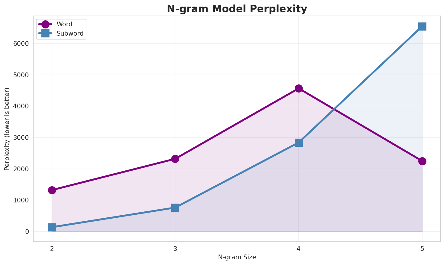
2. N-gram Model Evaluation

Results

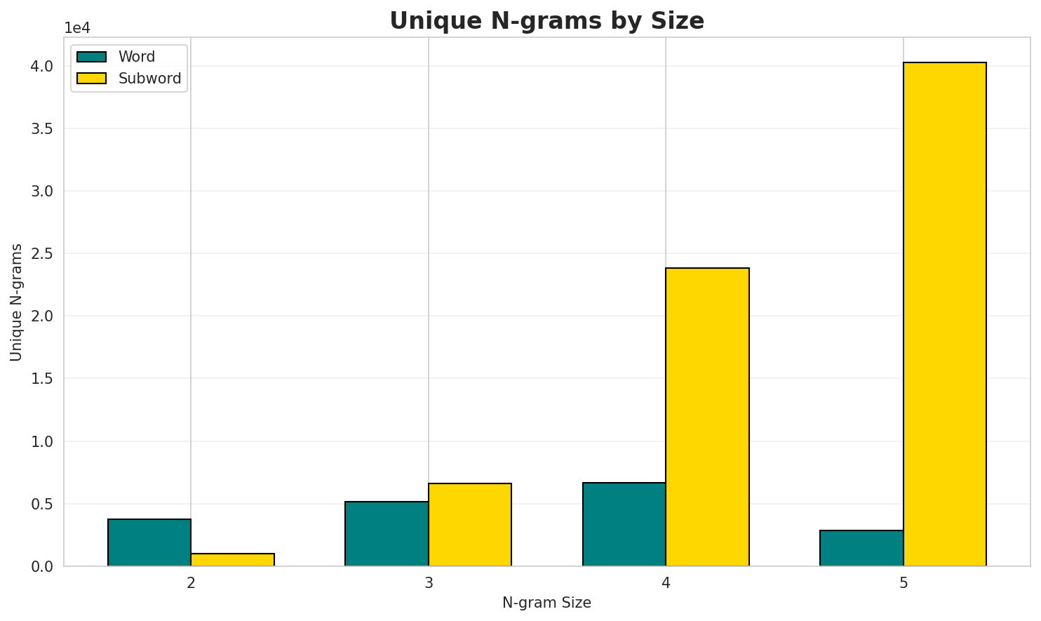
N-gram	Variant	Perplexity	Entropy	Unique N-grams	Top-100 Coverage	Top-1000 Coverage
2-gram	Word	1,320	10.37	3,772	35.4%	72.8%
2-gram	Subword	135 🏆	7.08	1,021	82.8%	100.0%
3-gram	Word	2,319	11.18	5,139	26.7%	58.4%
3-gram	Subword	762	9.57	6,635	47.4%	88.0%
4-gram	Word	4,567	12.16	6,660	15.3%	41.6%
4-gram	Subword	2,839	11.47	23,852	29.5%	65.9%
5-gram	Word	2,249	11.14	2,889	17.2%	54.1%
5-gram	Subword	6,549	12.68	40,232	20.3%	51.1%

Top 5 N-grams by Size

2-grams (Word):

Rank	N-gram	Count
1	dua na	2,793
2	e dua	1,910
3	kei na	1,768
4	na kena	1,059
5	mai na	875

3-grams (Word):

Rank	N-gram	Count
1	e dua na	1,710
2	me vaka na	432
3	ena dua na	337
4	e rawa ni	325
5	me baleta na	289

4-grams (Word):

Rank	N-gram	Count
1	kina e dua na	157
2	me vaka e dua	128
3	vaka e dua na	126
4	kei na dua na	94
5	dua vei ira na	94

5-grams (Word):

Rank	N-gram	Count
1	me vaka e dua na	118
2	tiko kina e dua na	81
3	e tiko kina e dua	61
4	e dua vei ira na	61
5	e dua na vanua ni	30

2-grams (Subword):

Rank	N-gram	Count
1	a _	58,970
2	i _	29,549
3	n a	29,239
4	_ n	27,570
5	k a	21,085

3-grams (Subword):

Rank	N-gram	Count
1	n a _	27,144
2	_ n a	17,261
3	a _ n	13,306
4	a k a	12,166
5	n i _	10,459

4-grams (Subword):

Rank	N-gram	Count
1	_ n a _	16,868
2	_ n i _	9,009
3	v a k a	8,886
4	a _ n a	8,331
5	_ v a k	7,039

5-grams (Subword):

Rank	N-gram	Count
1	a _ n a _	8,200
2	_ v a k a	6,983
3	i _ n a _	4,445
4	a _ n i _	4,282
5	_ e n a _	4,212

Key Findings

• Best Perplexity: 2-gram (subword) with 135
• Entropy Trend: Decreases with larger n-grams (more predictable)
• Coverage: Top-1000 patterns cover ~51% of corpus
• Recommendation: 4-gram or 5-gram for best predictive performance

---

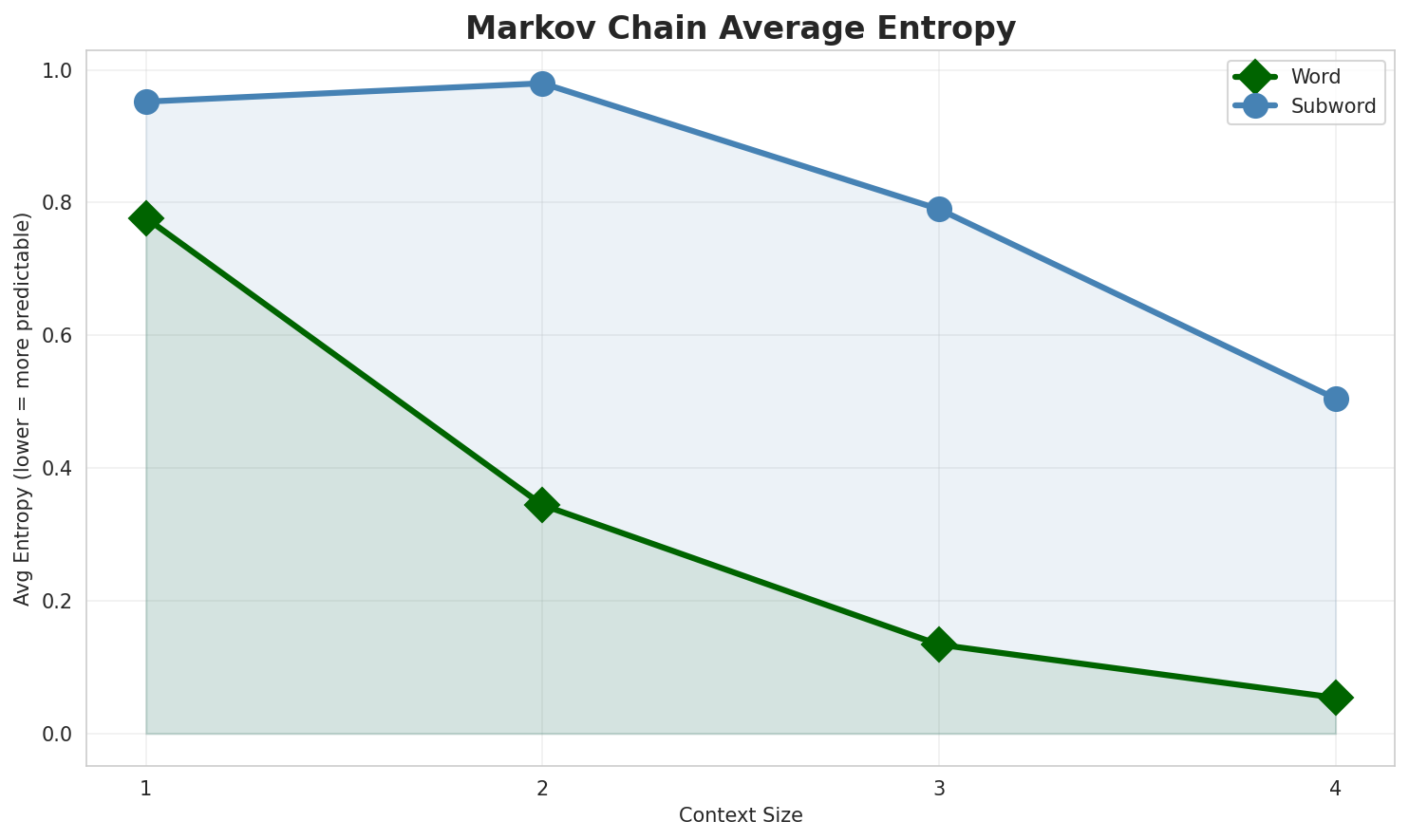
3. Markov Chain Evaluation

Results

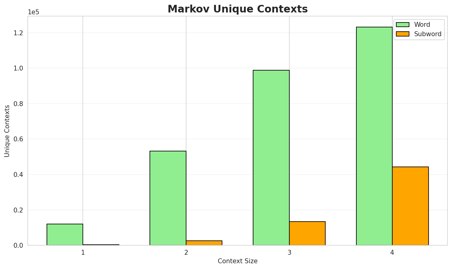
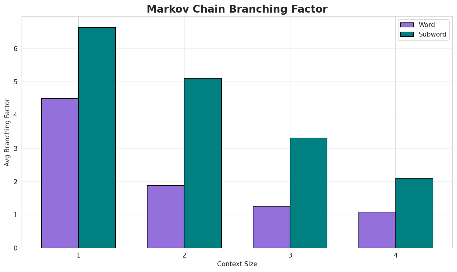
Context	Variant	Avg Entropy	Perplexity	Branching Factor	Unique Contexts	Predictability
1	Word	0.7768	1.713	4.51	11,967	22.3%
1	Subword	0.9522	1.935	6.63	397	4.8%
2	Word	0.3443	1.270	1.87	53,271	65.6%
2	Subword	0.9798	1.972	5.10	2,632	2.0%
3	Word	0.1340	1.097	1.26	98,857	86.6%
3	Subword	0.7901	1.729	3.31	13,399	21.0%
4	Word	0.0539 🏆	1.038	1.08	123,164	94.6%
4	Subword	0.5048	1.419	2.10	44,342	49.5%

Generated Text Samples (Word-based)

Below are text samples generated from each word-based Markov chain model:

Context Size 1:

1. na veikau se kavu epinephelus macrospilos epinephelus howlandi epinephelus species ni rerevaka na ma...
2. ni percussion ni tauyavutaki ena dua na koro levu ni potukali puerto la voui karisito oqo
3. e kune ena rawa e dua na kawatamata kena vakayagataki me vaka axial 82 23 mi

Context Size 2:

1. dua na tabana ka rawa me wainimate igu ia e dau yaco na veikau na uca kei
2. e dua na vanua e vakavuna na vakayalo ni veika vulavula e dua na lali e tu
3. kei na vakayagataki vakalevu me maroroi tikoga na kisi kei galileo ena lomanibai oqo e sega ni

Context Size 3:

1. e dua na sikorere ena matavuvale artamidae e sa vakaiyacaga sara ki na vuqa na itutu taudaku ni
2. me vaka na ena vuku ni dredre ni kena vakamacalataki na veimataqali vakasama ni bibi e tiko na
3. ena dua na koniteina vakauyaya ni sega ni tiko manumanu nodra sui e tiko ena yanuyanu o vanua

Context Size 4:

1. kina e dua na balavu ni ivakatagedegede e 2 7 ki 3 1 na gauna na kena titobu na
2. me vaka e dua na vanua ni wai ka drodro yani ena dela ni qele se na boto wasawasa
3. vaka e dua na droini mai vei rembrandt e dua na bula vakailavo e dua na vanua e 28

Generated Text Samples (Subword-based)

Below are text samples generated from each subword-based Markov chain model:

Context Size 1:

1. aki)_nuy_me_dreg
2. _enataromau_sita
3. iva_da,_raluqope

Context Size 2:

1. a_oqo_takarauta_y
2. i_ena_na_na_ni_ca
3. na_me_tuidini_va_

Context Size 3:

1. na_raraiti_e_dua_k
2. _na_vakasir_franx_
3. a_na_uciwaseinamat

Context Size 4:

1. _na_veiwale_e_vura_
2. _ni_sa_vakarai_na_t
3. vakaya_na_kai._rist

Key Findings

• Best Predictability: Context-4 (word) with 94.6% predictability
• Branching Factor: Decreases with context size (more deterministic)
• Memory Trade-off: Larger contexts require more storage (44,342 contexts)
• Recommendation: Context-3 or Context-4 for text generation

---

4. Vocabulary Analysis

Statistics

Metric	Value
Vocabulary Size	5,184
Total Tokens	136,582
Mean Frequency	26.35
Median Frequency	3
Frequency Std Dev	317.63

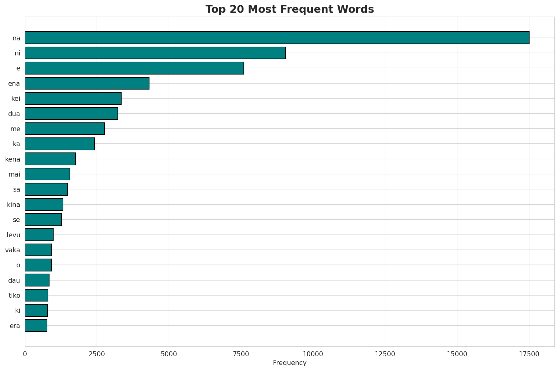
Most Common Words

Rank	Word	Frequency
1	na	17,507
2	ni	9,047
3	e	7,598
4	ena	4,309
5	kei	3,339
6	dua	3,228
7	me	2,753
8	ka	2,414
9	kena	1,753
10	mai	1,556

Least Common Words (from vocabulary)

Rank	Word	Frequency
1	pumona	2
2	ilatilati	2
3	cervix	2
4	movement	2
5	citations	2
6	translation	2
7	feminisimi	2
8	vakademografi	2
9	iceruniduka	2
10	balisi	2

Zipf's Law Analysis

Metric	Value
Zipf Coefficient	1.1690
R² (Goodness of Fit)	0.991059
Adherence Quality	excellent

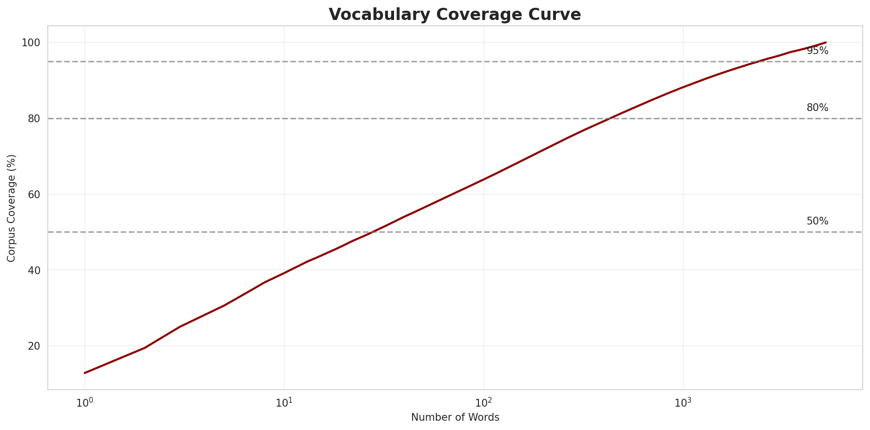
Coverage Analysis

Top N Words	Coverage
Top 100	63.9%
Top 1,000	88.2%
Top 5,000	99.7%
Top 10,000	0.0%

Key Findings

• Zipf Compliance: R²=0.9911 indicates excellent adherence to Zipf's law
• High Frequency Dominance: Top 100 words cover 63.9% of corpus
• Long Tail: -4,816 words needed for remaining 100.0% coverage

---

5. Word Embeddings Evaluation

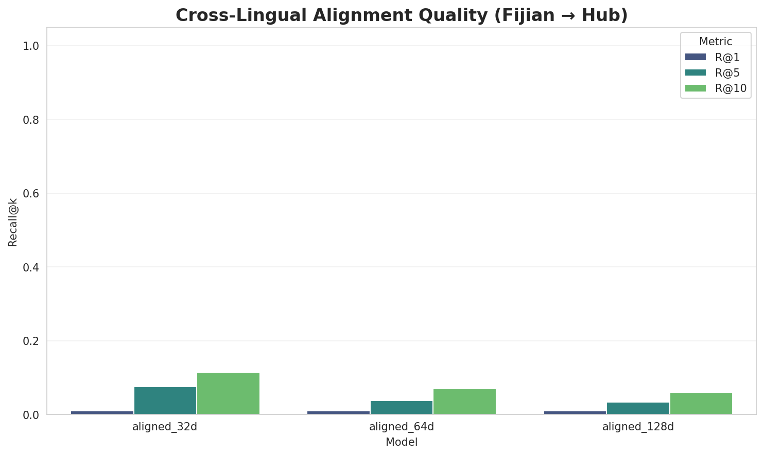
5.1 Cross-Lingual Alignment

5.2 Model Comparison

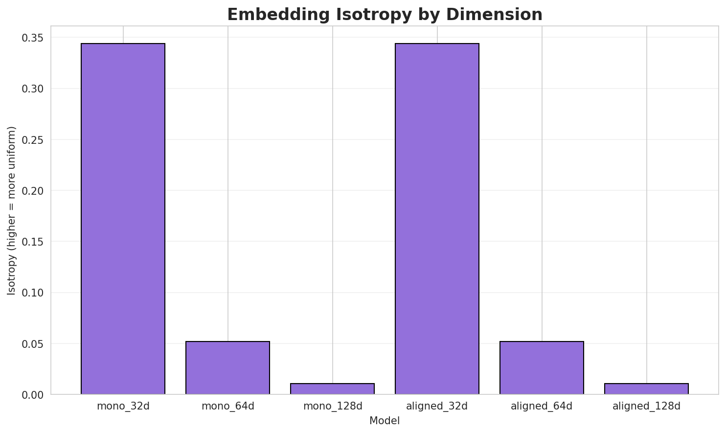
Model	Dimension	Isotropy	Semantic Density	Alignment R@1	Alignment R@10
mono_32d	32	0.3441 🏆	0.5376	N/A	N/A
mono_64d	64	0.0516	0.5508	N/A	N/A
mono_128d	128	0.0106	0.5737	N/A	N/A
aligned_32d	32	0.3441	0.5520	0.0100	0.1140
aligned_64d	64	0.0516	0.5538	0.0100	0.0700
aligned_128d	128	0.0106	0.5479	0.0100	0.0600

Key Findings

• Best Isotropy: mono_32d with 0.3441 (more uniform distribution)
• Semantic Density: Average pairwise similarity of 0.5526. Lower values indicate better semantic separation.
• Alignment Quality: Aligned models achieve up to 1.0% R@1 in cross-lingual retrieval.
• Recommendation: 128d aligned for best cross-lingual performance

---

6. Morphological Analysis (Experimental)

This section presents an automated morphological analysis derived from the statistical divergence between word-level and subword-level models. By analyzing where subword predictability spikes and where word-level coverage fails, we can infer linguistic structures without supervised data.

6.1 Productivity & Complexity

Metric	Value	Interpretation	Recommendation
Productivity Index	5.000	High morphological productivity	Reliable analysis
Idiomaticity Gap	0.058	Low formulaic content	-

6.2 Affix Inventory (Productive Units)

These are the most productive prefixes and suffixes identified by sampling the vocabulary for global substitutability patterns. A unit is considered an affix if stripping it leaves a valid stem that appears in other contexts.

Productive Prefixes

Prefix	Examples
-va	vakavuniwai, vakabauti, vakasamataki
-vak	vakavuniwai, vakabauti, vakasamataki
-vaka	vakavuniwai, vakabauti, vakasamataki
-ve	veikau, veitokoni, veibasai
-vei	veikau, veitokoni, veibasai
-ma	malea, makawa, matasawa

Productive Suffixes

Suffix	Examples
-a	ikoya, ijipita, república
-i	enijilisi, itaviqaravi, piqi
-ki	vakasamataki, vakayaloqaqataki, daramaki
-aki	vakasamataki, vakayaloqaqataki, daramaki
-ka	rawarataka, lifuka, taqomaka
-taki	vakasamataki, vakayaloqaqataki, yalataki
-ni	lesoni, sakini, nabavuni
-aka	rawarataka, taqomaka, marautaka

6.3 Bound Stems (Lexical Roots)

Bound stems are high-frequency subword units that are semantically cohesive but rarely appear as standalone words. These often correspond to the 'core' of a word that requires inflection or derivation to be valid.

Stem	Cohesion	Substitutability	Examples
atak	1.45x	18 contexts	mataka, vuataka, muataka
akat	1.41x	18 contexts	jakata, vakatui, vakatau
kata	1.34x	15 contexts	jakata, vakatau, vakatani
itak	1.41x	12 contexts	nuitaki, beitaki, kuitaki
akar	1.34x	12 contexts	vakaro, jakarta, vakarua
veiv	1.45x	9 contexts	veivala, veivola, veivula
eiva	1.50x	8 contexts	veivala, teivaka, teivaki
akav	1.36x	10 contexts	cakava, vakavo, rakavi
akac	1.47x	8 contexts	vakaca, vakacava, vakacegu
ivak	1.43x	8 contexts	teivaka, teivaki, ivakaro
amat	1.46x	7 contexts	tamata, squamata, matamata
kara	1.40x	7 contexts	karamu, ankara, vakarau

6.4 Affix Compatibility (Co-occurrence)

This table shows which prefixes and suffixes most frequently co-occur on the same stems, revealing the 'stacking' rules of the language's morphology.

Prefix	Suffix	Frequency	Examples
-va	-i	199 words	vakaoqori, vakaduri
-va	-a	186 words	vakatubura, vakawasoma
-ve	-i	126 words	veitiki, veitauni
-va	-ki	79 words	vakaituvakitaki, vakarerevaki
-va	-aki	75 words	vakaituvakitaki, vakarerevaki
-va	-taki	70 words	vakaituvakitaki, vakamatautaki
-va	-ka	58 words	vakatayaloyalotaka, vakasamataka
-ve	-ki	52 words	veitiki, veiwalitaki
-ve	-aki	48 words	veiwalitaki, veivakabulabulataki
-ve	-a	45 words	vekita, venezuela

6.5 Recursive Morpheme Segmentation

Using Recursive Hierarchical Substitutability, we decompose complex words into their constituent morphemes. This approach handles nested affixes (e.g., prefix-prefix-root-suffix).

Word	Suggested Split	Confidence	Stem
veivosakitaki	vei-vosa-ki-taki	7.5	vosa
vakaikuritaki	vaka-ikuri-taki	6.0	ikuri
veivosaki	vei-vosa-ki	6.0	vosa
vakatikina	vaka-tiki-na	6.0	tiki
vakabulabulataki	vaka-bulabula-taki	6.0	bulabula
vakatututaki	vaka-tutu-taki	6.0	tutu
vakasucuna	vaka-sucu-na	6.0	sucu
veiyasana	vei-yasa-na	6.0	yasa
vakagalalataki	vaka-galala-taki	6.0	galala
vakalewena	vaka-lewe-na	6.0	lewe
vakawaicalataki	vaka-waicala-taki	6.0	waicala
vakaduiduitaki	vaka-duidui-taki	6.0	duidui
vakadodonutaki	vaka-dodonu-taki	6.0	dodonu
veitinani	vei-tina-ni	6.0	tina
veitacini	vei-taci-ni	6.0	taci

6.6 Linguistic Interpretation

Automated Insight: The language Fijian shows high morphological productivity. The subword models are significantly more efficient than word models, suggesting a rich system of affixation or compounding.

---

7. Summary & Recommendations

Production Recommendations

Component	Recommended	Rationale
Tokenizer	32k BPE	Best compression (4.56x)
N-gram	2-gram	Lowest perplexity (135)
Markov	Context-4	Highest predictability (94.6%)
Embeddings	100d	Balanced semantic capture and isotropy

---

Appendix: Metrics Glossary & Interpretation Guide

This section provides definitions, intuitions, and guidance for interpreting the metrics used throughout this report.

Tokenizer Metrics

Compression Ratio

Definition: The ratio of characters to tokens (chars/token). Measures how efficiently the tokenizer represents text.

Intuition: Higher compression means fewer tokens needed to represent the same text, reducing sequence lengths for downstream models. A 3x compression means ~3 characters per token on average.

What to seek: Higher is generally better for efficiency, but extremely high compression may indicate overly aggressive merging that loses morphological information.

Average Token Length (Fertility)

Definition: Mean number of characters per token produced by the tokenizer.

Intuition: Reflects the granularity of tokenization. Longer tokens capture more context but may struggle with rare words; shorter tokens are more flexible but increase sequence length.

What to seek: Balance between 2-5 characters for most languages. Arabic/morphologically-rich languages may benefit from slightly longer tokens.

Unknown Token Rate (OOV Rate)

Definition: Percentage of tokens that map to the unknown/UNK token, indicating words the tokenizer cannot represent.

Intuition: Lower OOV means better vocabulary coverage. High OOV indicates the tokenizer encounters many unseen character sequences.

What to seek: Below 1% is excellent; below 5% is acceptable. BPE tokenizers typically achieve very low OOV due to subword fallback.

N-gram Model Metrics

Perplexity

Definition: Measures how "surprised" the model is by test data. Mathematically: 2^(cross-entropy). Lower values indicate better prediction.

Intuition: If perplexity is 100, the model is as uncertain as if choosing uniformly among 100 options at each step. A perplexity of 10 means effectively choosing among 10 equally likely options.

What to seek: Lower is better. Perplexity decreases with larger n-grams (more context). Values vary widely by language and corpus size.

Entropy

Definition: Average information content (in bits) needed to encode the next token given the context. Related to perplexity: perplexity = 2^entropy.

Intuition: High entropy means high uncertainty/randomness; low entropy means predictable patterns. Natural language typically has entropy between 1-4 bits per character.

What to seek: Lower entropy indicates more predictable text patterns. Entropy should decrease as n-gram size increases.

Coverage (Top-K)

Definition: Percentage of corpus occurrences explained by the top K most frequent n-grams.

Intuition: High coverage with few patterns indicates repetitive/formulaic text; low coverage suggests diverse vocabulary usage.

What to seek: Depends on use case. For language modeling, moderate coverage (40-60% with top-1000) is typical for natural text.

Markov Chain Metrics

Average Entropy

Definition: Mean entropy across all contexts, measuring average uncertainty in next-word prediction.

Intuition: Lower entropy means the model is more confident about what comes next. Context-1 has high entropy (many possible next words); Context-4 has low entropy (few likely continuations).

What to seek: Decreasing entropy with larger context sizes. Very low entropy (<0.1) indicates highly deterministic transitions.

Branching Factor

Definition: Average number of unique next tokens observed for each context.

Intuition: High branching = many possible continuations (flexible but uncertain); low branching = few options (predictable but potentially repetitive).

What to seek: Branching factor should decrease with context size. Values near 1.0 indicate nearly deterministic chains.

Predictability

Definition: Derived metric: (1 - normalized_entropy) × 100%. Indicates how deterministic the model's predictions are.

Intuition: 100% predictability means the next word is always certain; 0% means completely random. Real text falls between these extremes.

What to seek: Higher predictability for text generation quality, but too high (>98%) may produce repetitive output.

Vocabulary & Zipf's Law Metrics

Zipf's Coefficient

Definition: The slope of the log-log plot of word frequency vs. rank. Zipf's law predicts this should be approximately -1.

Intuition: A coefficient near -1 indicates the corpus follows natural language patterns where a few words are very common and most words are rare.

What to seek: Values between -0.8 and -1.2 indicate healthy natural language distribution. Deviations may suggest domain-specific or artificial text.

R² (Coefficient of Determination)

Definition: Measures how well the linear fit explains the frequency-rank relationship. Ranges from 0 to 1.

Intuition: R² near 1.0 means the data closely follows Zipf's law; lower values indicate deviation from expected word frequency patterns.

What to seek: R² > 0.95 is excellent; > 0.99 indicates near-perfect Zipf adherence typical of large natural corpora.

Vocabulary Coverage

Definition: Cumulative percentage of corpus tokens accounted for by the top N words.

Intuition: Shows how concentrated word usage is. If top-100 words cover 50% of text, the corpus relies heavily on common words.

What to seek: Top-100 covering 30-50% is typical. Higher coverage indicates more repetitive text; lower suggests richer vocabulary.

Word Embedding Metrics

Isotropy

Definition: Measures how uniformly distributed vectors are in the embedding space. Computed as the ratio of minimum to maximum singular values.

Intuition: High isotropy (near 1.0) means vectors spread evenly in all directions; low isotropy means vectors cluster in certain directions, reducing expressiveness.

What to seek: Higher isotropy generally indicates better-quality embeddings. Values > 0.1 are reasonable; > 0.3 is good. Lower-dimensional embeddings tend to have higher isotropy.

Average Norm

Definition: Mean magnitude (L2 norm) of word vectors in the embedding space.

Intuition: Indicates the typical "length" of vectors. Consistent norms suggest stable training; high variance may indicate some words are undertrained.

What to seek: Relatively consistent norms across models. The absolute value matters less than consistency (low std deviation).

Cosine Similarity

Definition: Measures angular similarity between vectors, ranging from -1 (opposite) to 1 (identical direction).

Intuition: Words with similar meanings should have high cosine similarity. This is the standard metric for semantic relatedness in embeddings.

What to seek: Semantically related words should score > 0.5; unrelated words should be near 0. Synonyms often score > 0.7.

t-SNE Visualization

Definition: t-Distributed Stochastic Neighbor Embedding - a dimensionality reduction technique that preserves local structure for visualization.

Intuition: Clusters in t-SNE plots indicate groups of semantically related words. Spread indicates vocabulary diversity; tight clusters suggest semantic coherence.

What to seek: Meaningful clusters (e.g., numbers together, verbs together). Avoid over-interpreting distances - t-SNE preserves local, not global, structure.

General Interpretation Guidelines

1. Compare within model families: Metrics are most meaningful when comparing models of the same type (e.g., 8k vs 64k tokenizer).
2. Consider trade-offs: Better performance on one metric often comes at the cost of another (e.g., compression vs. OOV rate).
3. Context matters: Optimal values depend on downstream tasks. Text generation may prioritize different metrics than classification.
4. Corpus influence: All metrics are influenced by corpus characteristics. Wikipedia text differs from social media or literature.
5. Language-specific patterns: Morphologically rich languages (like Arabic) may show different optimal ranges than analytic languages.

Visualizations Index

Visualization	Description
Tokenizer Compression	Compression ratios by vocabulary size
Tokenizer Fertility	Average token length by vocabulary
Tokenizer OOV	Unknown token rates
Tokenizer Total Tokens	Total tokens by vocabulary
N-gram Perplexity	Perplexity by n-gram size
N-gram Entropy	Entropy by n-gram size
N-gram Coverage	Top pattern coverage
N-gram Unique	Unique n-gram counts
Markov Entropy	Entropy by context size
Markov Branching	Branching factor by context
Markov Contexts	Unique context counts
Zipf's Law	Frequency-rank distribution with fit
Vocab Frequency	Word frequency distribution
Top 20 Words	Most frequent words
Vocab Coverage	Cumulative coverage curve
Embedding Isotropy	Vector space uniformity
Embedding Norms	Vector magnitude distribution
Embedding Similarity	Word similarity heatmap
Nearest Neighbors	Similar words for key terms
t-SNE Words	2D word embedding visualization
t-SNE Sentences	2D sentence embedding visualization
Position Encoding	Encoding method comparison
Model Sizes	Storage requirements
Performance Dashboard	Comprehensive performance overview

---

About This Project

Data Source

Models trained on wikipedia-monthly - a monthly snapshot of Wikipedia articles across 300+ languages.

Project

A project by Wikilangs - Open-source NLP models for every Wikipedia language.

Maintainer

Omar Kamali - Omneity Labs

Citation

If you use these models in your research, please cite:

@misc{wikilangs2025,
  author = {Kamali, Omar},
  title = {Wikilangs: Open NLP Models for Wikipedia Languages},
  year = {2025},
  doi = {10.5281/zenodo.18073153},
  publisher = {Zenodo},
  url = {https://huggingface.co/wikilangs}
  institution = {Omneity Labs}
}

License

MIT License - Free for academic and commercial use.

Links

• 🌐 Website: wikilangs.org
• 🤗 Models: huggingface.co/wikilangs
• 📊 Data: wikipedia-monthly
• 👤 Author: Omar Kamali
• 🤝 Sponsor: Featherless AI

---

Generated by Wikilangs Models Pipeline

Report Date: 2026-01-04 14:43:20